 |
GemaMesh
The GeMA Mesh Plugin
|
Loading...
Searching...
No Matches
|
GemaMesh
The GeMA Mesh Plugin
|
The GemaMesh plugin publishes three main object types that can be used while providing the mesh type name. They are:
Besides, three additional object types, GemaMesh.nodesd, GemaMesh.celld and GemaMesh.elemd are available. Their capabilities are exactly the same as their "no d" brothers. The difference is that mesh data storage is specially tailored for situations where new nodes and cells will be continuouslly added to the mesh in an incremental way during the simulation. For the "d" types, a dual vector structure is adopted. The first part stores the, fixed, original mesh data, while the incrementally added nodes, cells and their data are stored at the second part. With the said partition, only the (hopefully small) second vectors need to be grown as new cells are added to the mesh. The cost of this separation is the need for a behind the scenes conditional clause to check which part of the vector should be used when accesing data.
When defining a Gema Mesh object, the following fields are available for usage during the definition:
| Attribute | Description | Type | Required |
|---|---|---|---|
| id | The mesh name. | String | Yes |
Example: id = "myMeshName" | |||
| typeName | Mesh plugin name. Should be equal to 'GemaMesh.xxx', where xxx = nodes, cell or elem. | String | Yes |
Example: typeName = "GemaMesh.elem" | |||
| description | An optional description of the mesh purpose. | String | No |
Example: description = "Discretized 100x100 plate" | |||
| dumpFile | If this option is given, the mesh geometry and initial values will be loaded from the given dump file. The file stored mesh must have the same meta-data as the one described in this mesh. In particular, the set of state-variables, attribtes and property sets must be the same. See comments on the State dump documentation. When using this option, the nodeData, ghostData, cellData, nodeSetData, cellGroupData, boundaryEdgeData and boundaryFaceDatafields should not be filled since their contents will be read from the dump file. This can greatlly speed up the mesh loading process. | String | No |
Example: dumpFile = "$SIMULATIONDIR/$SIMULATIONNAME.dmp" | |||
| hdf5File | Similar to dumpFile but reading data from a .gh5 file. This is an HDF5 file with GeMA mesh data. It can have been created by an external pre-processor or by a call to io.saveToHdf5ModelFile(). | String | No |
Example: hdf5File = "$SIMULATIONDIR/$SIMULATIONNAME.gh5" | |||
| coordinateDim | The number of dimensions for each node coordinate. Should be a value equal to 1, 2 or 3. | Integer | Yes |
Example: coordinateDim = 2 | |||
| coordinateUnit | The optional unit in which node coordinates are expressed. The default value is the empty string, which is compatible with any unit system. See also the documentation on Working with units. | String | No |
Example: coordinateUnit = "m" | |||
| coordinateFormat | This optional field controls how coordinate values will be formatted when printed or saved to a text file format. It uses a subset of the C printf() syntax, allowing the user to specify the field width, precision and format type. A format = "8.2f" statement means that the formatted value will have at least 8 characters and 2 decimal values. Allowed format specifiers are 'f' (for decimal floating point format), 'e' (for scientific notation format) and 'g' (corresponding to 'f' or 'e', whichever is shortest). Default = "12.2f". | String | No |
Example: coordinateFormat = "6.3f" | |||
| topology | An optional flag that when set to true instructs GeMA to build the additional data structure used for topological queries just after loading the mesh data. Setting this flag to true is not needed for performing topological queries since the structure will be built at the first time that it is needed, but can make sure that it is built in a more predictable moment. | Boolean | No |
Example: topology = true | |||
| topologyBuildEdgeMap | An optional flag that when set to true instructs GeMA to include an "edge -> half-face" map in the topological structure for solid meshes. This map is used by edge queries performed over solid meshes (but is not required for them to work). Since it consumes much more memory than the whole rest of the structure, it is not created by default. | Boolean | No |
Example: topologyBuildEdgeMap = true | |||
| topologyCheckOptions | An optional attribute that controls the level of checking that is done when building the topology structure. Possible values are: - "basic": Only performs trivial, no cost, checks while the structure is built. - "simple": Performs additional checks over the opposite tables. Can usually detect most problems on a mesh. - "full": Performs the same checks that the simple mode and also checks, for each node, if the adjacent cells query is correct. Should be able to detect any non-manifold problems with the mesh (excludes "strange" elements from the test - bar elements from surface meshes or bar and surface elements from solid meshes). - "basic warn", "simple warn" and "full warn": Same as the no warn version, but considers any problems as warnings and not errors. The topology structure will be built but might be unreliable for some queries. The deault is "basic" and can be changed by the gema configuration option with the same name. | String | No |
Example: topologyCheckOptions = "full" | |||
| singleCellType | An optional flag that when set to true tells GeMA that all the mesh cells have a single type, and more importantly, that no cells with a different type will be added later to the mesh. This has an effect of allowing GeMA to perform some space optimizations when creating the topological data structure. If this flag is set to true, an error will be raised if an attempt is made to add a new cell to the mesh with type different from the existing cells. | Boolean | No |
Example: singleCellType = true | |||
| useGhostNodes | An optional flag controlling if the mesh supports ghost nodes or not. If set to false, no support for ghost nodes will exist for state variables and node attributes tied to this mesh, even if they request so through the storage field. Default = false. | Boolean | No |
Example: useGhostNodes = true | |||
| hOrder | A table that should be filled only when the mesh contains hierarchical elements, such as hquadp or hhexp. When given, it should be a table with fields P and Q, storing, respectively, the requested polynomial orders for scalar and vector fields. This option automatically implies in useGhostNodes = true. Keep in mind that although meshes can store heterogeneous elements, all of them must be either hierarchical or not. Mixing them is not possible. | Table | No |
Example: hOrder = {P = 3, Q = 2} | |||
| stateVars | A table with the list of the ids of the state variables that will be stored in mesh nodes and/or cells. Can include node state variables, cell state variables or both. Although optional (a mesh can be created without being associated with state variables), it is required by most physics plugins. | Table | No |
Example: stateVars = { "u", "p" } | |||
| cellProperties | A table with the list of the ids of the property sets that will be associated with this mesh. Each mesh cell / element will store a line index for each associated property set. Ignored for node meshes. Although optional for cell and element meshes, (a mesh can be created without being associated with a property set), it is required by most physics plugins. | Table | No |
Example: cellProperties = { "MateriaPropertySet" } | |||
| nodeAttributes | An optional table with the definition of the attributes associated with mesh nodes. Each table entry is a sub-table with a node attribute defintion following the syntax described in the Data options page. | Table | No |
Example: nodeAttributes = { { id = "nodeAttr1", description = "Sample scalar node attribute", unit = "g/cm3" }, { id = "nodeAttr2", dim = 2, description = "Sample vector node attribute" }, } | |||
| cellAttributes | An optional table with the definition of the attributes associated with mesh cells / elements. Each table entry is a sub-table with a cell attribute defintion following the syntax described in the Data options page. Ignored for node meshes. | Table | No |
Example: cellAttributes = { { id = "cellAttr1", description = "Sample scalar cell attribute", unit = "g/cm3" }, { id = "cellAttr2", dim = 2, description = "Sample vector cell attribute" }, } | |||
| gaussAttributes | An optional table with the definition of the attributes associated with mesh element integration points. Each table entry is a sub-table with a Gauss attribute defintion following the syntax described in the Data options page. When working with multiple integration rules, don't forget to specify the desired ruleSet. Ignored for node and cell meshes. | Table | No |
Example: gaussAttributes = { { id = "gaussAttr1", description = "Sample scalar Gauss attribute", unit = "g/cm3" }, { id = "gaussAttr2", dim = 2, description = "Sample vector Gauss attribute", ruleSet = 2 }, } | |||
| nodeData | A table storing node information for the mesh. This table has one sub-table for each node, storing, in this order, the node coordinates, optionally followed by node attribute and node state var initial values. See the Node data section below for details. Alternatively, this field can be a Lua function that when called without parameters returns the number of mesh nodes, and when called with an index 'i' returns the 'ith' node sub-table. The function will be called once without parameters and then once for each node ('i' varying from 1 to the number of nodes). It also supports receiving a table filled with several sub-tables, formated as above, that will be concatenated by the mesh loader as if they where a single node table. | Table or function | Yes |
Example: nodeData = { {0.0, 0.0}, {1.0, 0.0}, {2.0, 0.0}, {0.0, 1.0}, {1.0, 1.0}, {2.0, 1.0} } for a 2D mesh with 6 nodes where only the coordinates where initialized. See the global example below for a more elaborate scenario. | |||
| ghostData | A table (or function) similar to nodeData, storing ghost node coordinates, attributes and state var initial values. Attribute and state var values are optional. Details on the Node data section below are also applicable to ghostData. This field will be parsed only if useGhostNodes is true. | Table or function | No |
| Example: See the global example below for a more elaborate scenario. | |||
| cellData | A table storing cell types, conectivity information, groupings and initial attribute, cell state var and property values. Each table entry is a sub-table storing information about a group of cells of the same type. Ignored for node meshes. It contains the following subfields: - cellType: A string defining the type of the cells stored in cellList for this entry. The mesh can contain elements with different types but they must be separated in different entries since all the elements in cellList must share the same type. - cellGroup: The optional name of the group that this cells belongs to. Different table entries with same group name are merged in the same group by the reader. - xxx: When 'xxx' equals the name of a property set included in cellProperties, this field value will be the default property index associated with cells in cellList that do not explicitly overrides this default. A property index can reference a property set line either by an integer index or an id name. If a mesh is associated with several property sets, in general it should include one default value for each property set, otherwise, that property set value MUST be provided for each cell in cellList since every cell must be connected with a property set line for each property set attached to the mesh. - cellList: The list of element conectivity, cell attribute and state variable initial values and property set index assignments. This list is a table with an entry for each cell of this cellType/cellGroup, containing, in this order, the set of node numbers that define the cell, respecting the cell type prescribed order, optionally followed by cell attribute initial values and cell state variable initial values. Property set index values should be given by a named (property set, index) pair. They are optional only if a default association was included in the table that hosts this cell list. If useGhostNodes is set to true, a special key ghostNodes can optionally receive a table with a set of cell ghost node indices that will be included in the cell definition. See the Cell data section below for details. Alternatively, this subfield can be a Lua function that when called without parameters returns the number of mesh cells in this group, and when called with an index 'i' returns the 'ith' cell sub-table. The function will be called once without parameters and then once for each cell ('i' varying from 1 to the number of cells). | Table | Yes for cell and element meshes |
Example: cellData = { { cellType = "quad4", MaterialPropertySet = 1, cellList = {{1, 2, 5, 4}, {2, 3, 6, 5, MaterialPropertySet = 2}} } } for a mesh with only two cells in a single group, no cell initialization and a single property set. See the global example below for a more elaborate scenario. | |||
| elementRules | An optional table defining the set of available integration rule sets for this mesh elements. Each table entry is a sub-table with one rule set definition. Rule sets are used for defining the number of integration points used by FEM physics objects and for defining the number of Gauss points in a Gauss attribute. Each rule set consists in a set of pairs associating element type names with a rule that can be given as a number or a string. The value quad4 = 3, associates quad4 elements with a 3 x 3 element integration rule while quad4 = '3x2' to a anisotropic rule with 3 points along the element horizontal direction and 2 along its vertical direction. Similarly, hex8 = 3, associates hex8 elements with a 3 x 3 x 3 rule while hex8 = '3x4x5' to a anisotropic rule. An optional prefix letter can be used to specify the type of integration rule. Available options are G or g for Gauss rules, N, n, CN, cn, ON or on for closed or open Newton-Cotes rules (the N or n options are analogue to CN) and L or l for Lobatto rules. If this type specifier is missing, the default for the element type will be used (see the Element types documentation). If an element type is not present in the rule set, or an invalid rule is specified, its default rule will be assumed. It really only makes sense to add to a rule set element types used in the mesh. Also, keep in mind that rule sets are needed only when there is a desire to depart from the default rules for an elment type. Ignored for node and cell meshes. | Table | No |
Example: elementRules = { {quad4 = 2, tri3 = 1}, -- Rule set 1 {quad4 = 3, tri3 = 3}, -- Rule set 2 {quad4 = "L5x3", tri3 = "G3"}, -- Rule set 3 } | |||
| faceRules | An optional table, similar in purpose and following the same general syntax as elementRules, providing the rules used when integrating over an element face. Should include rules for 3D element types only. In general, this table size should be equal to the elementRules table size since they both reference the same rule set (when a physics object or a Gauss attribute specifies a rule set, it is selecting a row from both tables). If a rule set exists in one table and not in the other, the missing rule set will be considered as using default values for each type, so it is possible to have one table without the other. Ignored for node and cell meshes. For 3D elements with multiple face types, like a wedge6 whose faces can be either triangles or quadrilaterals, the element name should be suffixed with the face type name (either _quad or _tri) for defining the specific rule for each face type. | Table | No |
Example: faceRules = { {hex8 = "2x2", tet4 = 3, wedge6_quad = "2x2", wedge6_tri = 3}, -- Rule set 1 {hex8 = 3, tet4 = 6, wedge6_quad = 3, wedge6_tri = 6}, -- Rule set 2 } | |||
| edgeRules | An optional table, similar in purpose and following the same syntax as elementRules, providing the rules used when integrating over an element edge. Can include rules for both 2D and 3D elements. In general, this table size should be equal to the elementRules table size since they both reference the same rule set (when a physics object or a Gauss attribute specifies a rule set, it is selecting a row from both tables). If a rule set exists in one table and not in the other, the missing rule set will be considered as using default values for each type, so it is possible to have one table without the other. Ignored for node and cell meshes. | Table | No |
Example: edgeRules = { {quad4 = 2, tri3 = 1}, -- Rule set 1 {quad4 = 3, tri3 = 1}, -- Rule set 2 } | |||
| nodeSetData | An optional table storing a set of named collections of mesh nodes. Each table entry is a sub-table that stores an id with the node set name and a node list where each entry is a mesh node number. Ghost numbers can be included in the table as negative numbers (a value of -2 represents the second ghost number in the ghostData table). Alternatively, the nodeList subfield can be a Lua function that when called without parameters returns the number of nodes in this node set, and when called with an index 'i' returns the 'ith' node. The function will be called once without parameters and then once for each node ('i' varying from 1 to the number of nodes). It can also be a cell group name (see the cellData documentation). In that case, the node set will be filled with the set of geometry nodes referenced by the cells in the named group. | Table | No |
Example: nodeSetData = { { id = "top nodes", nodeList = { 4, 5, -3, 6} }, -- Nodes 4, 5 and 6 + Ghost node 3 { id = "left nodes", nodeList = { 1, 4 } }, -- Nodes 1 and 4 { id = "group nodes", nodeList = "cell group name"}, -- Nodes referenced by cells in the named cell group } | |||
| cellGroupData | An optional table storing a set of named collections of cells that will be merged with the cell groups defined in the cellData table. Notice that entries from this table should represent new cell groups. Each table entry is a sub-table that stores an id with the cell group name and a cell list where each entry is a cell number. Alternatively, the cellList subfield can be a Lua function that when called without parameters returns the number of entries in this group, and when called with an index 'i' returns the 'ith' cell. The function will be called once without parameters and then once for each entry ('i' varying from 1 to the number of entries). The cell list can be replaced by a filter function given by extractFilter. This function is applied over mesh cells and defines which of those cells will make into the named group. See the Filter functions section below for details. | Table | No |
Example: cellGroupData = { { id = "group 1", cellList = { 8, 9, 13, 20} }, -- Explicitely defined cells { id = "group 2", extractFilter = function(d) return d.ps_mat == 2 end}, -- Cells whose property set "mat" index are equal to 2 } | |||
| boundaryEdgeData | An optional table storing a set of named collections of cell borders. Each table entry is a sub-table that stores an id with the boundary name and a cell list where each entry is another table with a cell id and a border id inside this cell. See the Element types documentation for a reference about border numbering for the available mesh cell types. See the Boundary data section below for details. Ignored for node meshes. Alternatively, the cellList subfield can be a Lua function that when called without parameters returns the number of entries in this border, and when called with an index 'i' returns the 'ith' cell/border sub-table. The function will be called once without parameters and then once for each entry ('i' varying from 1 to the number of entries). If the mesh is a surface mesh, the cell list can be replaced by a filter function given by extractFilter. This function is applied over mesh border edges and defines which of those edges will make into the named boundary. See the Filter functions section below for details. If the function is present, the extractBorder field can be used to further narrow the set of candidate edges. Its value can be either a border index or a table with a cell id + border index from an edge belonging to the desired border. In that case, the extract function will only be called for edges on that border. | Table | No |
Example: boundaryEdgeData = { { id = "top border", cellList = { {1, 3}, {2, 3} } }, -- Element 1, border 3 + element 2, border 3 { id = "bottom border", cellList = { {1, 1}, {2, 1} } }, -- Element 1, border 1 + element 2, border 1 { id = "left border", extractFilter = function(d) return d.normal(1) < -0.99 end }, -- All edges whose normal vector point on the negative X direction { id = "left border", extractFilter = function(d) return d.normal(1) < -0.99 end, extractBorder = {1, 3} }, -- Same as above but the function is only called for edges from the border containing cell 1, edge 3. } | |||
| boundaryFaceData | An optional table, following the same syntax as boundaryEdgeData, but storing face ids instead of border ids. See the Boundary data section below for details. If an extract filter is given, it will be applied over border faces. See the Filter functions section below for details. Ignored for node meshes. | Table | No |
Example: boundaryFaceData = { { id = "top face", cellList = { {1, 5} } } -- Element 1, face 5 { id = "right faces", extractFilter = function(d) return d.normal(1) > 0.99 end }, -- All faces whose normal vector point on the positive X direction } | |||
As explained above, each entry in the nodeData table is a table containing node coordinates, optionally followed by initial values for node attributes and node state variables. Those values must follow first the definition order in the nodeAttributes table and then the definition order for node state variables in the stateVars table.
Likewise, the cellList inside the cellData table can include cell attribute initial values and cell state variables. Those values must follow first the definition order in the cellAttributes table and then the definition order for cell state variables in the stateVars table. The syntax is the same for both node and cell data initialization.
All initial values are optional, but for one value to be present, all previous values should also be present (or a nil should be given in its place). Trailing nil values can be ommited. If a value is not present, or a nil value is provided as initial value, the attribute / state variable default value will be used (if its declaration does not include a defVal clause, 0.0 will be used).
Values are expected to be in the unit given on the attribute / state variable declaration. Vector values should be given as a Lua table. For matrices, the initial value can be either given by a table of tables or linearized by column major format (the same used in the FORTRAN language), so, for a 2x2 matrix, both {11, 21, 12, 22} and { {11, 12}, {21, 22} } statements correspond to the matrix \(\begin{pmatrix} 11 & 12 \\ 21 & 22 \end{pmatrix}\). If an attribute supports functions, the value can also be a string with a function name.
Node and cell initialization example:
The resulting initial values for the above mesh nodes and cells are (bold values are default values replacing a nil or a missing value):
| node | x | y | na1 | na2 | na3 | sv1 | sv2 |
|---|---|---|---|---|---|---|---|
| 1 | 0 | 0 | 5.7 | {0.45, 1.23} | {{11.1, 12.1}, {21.1, 22.1}} | {101.0, 101.1, 101.2} | 1.1 |
| 2 | 10 | 0 | 5.8 | {0.00, 0.00} | {{11.0, 12.0}, {21.0, 22.0}} | {102.0, 102.1, 102.2} | 0.0 |
| 3 | 20 | 0 | -999 | {0.47, 1.25} | {{11.0, 12.0}, {21.0, 22.0}} | { 0.0, 0.0, 0.0} | 0.0 |
| 4 | 0 | 10 | 'f' | {0.48, 1.26} | {{11.4, 12.4}, {21.4, 22.4}} | {201.0, 201.1, 201.2} | 2.1 |
| 5 | 10 | 10 | -999 | {0.00, 0.00} | {{11.0, 12.0}, {21.0, 22.0}} | { 0.0, 0.0, 0.0} | 0.0 |
| cell | incidence | ca1 | csv1 |
|---|---|---|---|
| 1 | 1, 2, 5, 4 | 15.7 | 3.14 |
| 2 | 1, 3, 5, 4 | 18.2 | 6.27 |
As explained above, each entry in the cellList table inside a boundaryEdgeData or boundaryFaceData tables contains pairs with node ids and border / face numbers. Border and face number ordering can be found on the Element types documentation. The following example shows how to define edge borders for the top and left borders for the mesh on the image below, where cell numbers are shown for each cell, and border edge numbers for cell 2.
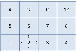
Important: edge numbering depends on the order that nodes where listed when defining a cell. For a quad element, the first edge will always be between the first and second cell nodes, but the location of that border (top, bottom, left or right for an axis aligned quad) depends on the order that the nodes where given. On the image below, the numbers in the cell corners are the order in which each node appears in the cell definition, and the numbers along lines the edge numbers.

Filter functions are a way to define cell groups, edge boundaries or face boundaries without the need for manually listing each cell / border with cellList entries inside the cellGroupData, boundaryEdgeData or boundaryFaceData tables. They are defined through the extractFilter entry, which should provide a function that receives a single table d as parameter and returns true if the given cell / border (edge or face) should be added to the group / boundary, or false if not.
When applied to select cells for a group, the given function is called for every cell in the mesh with the d parameter containing a description of the cell to be accepted or rejected. When applied to provide edges for a surface mesh or faces for a volumetric mesh, it is called for every edge / cell in the mesh border, with the d parameter containing a description of the cell edge or face to be accepted or rejected. In the later case, if the extractFilter function is matched by an extractBorder field, the function will be called only for edges / faces that belong to the specified mesh border, either directly through a border index or indirectly through the description of an edge / face in the border (given by a cell + border index pair). The d parameter is a standard Lua table. The available fields in this table are detailed below.
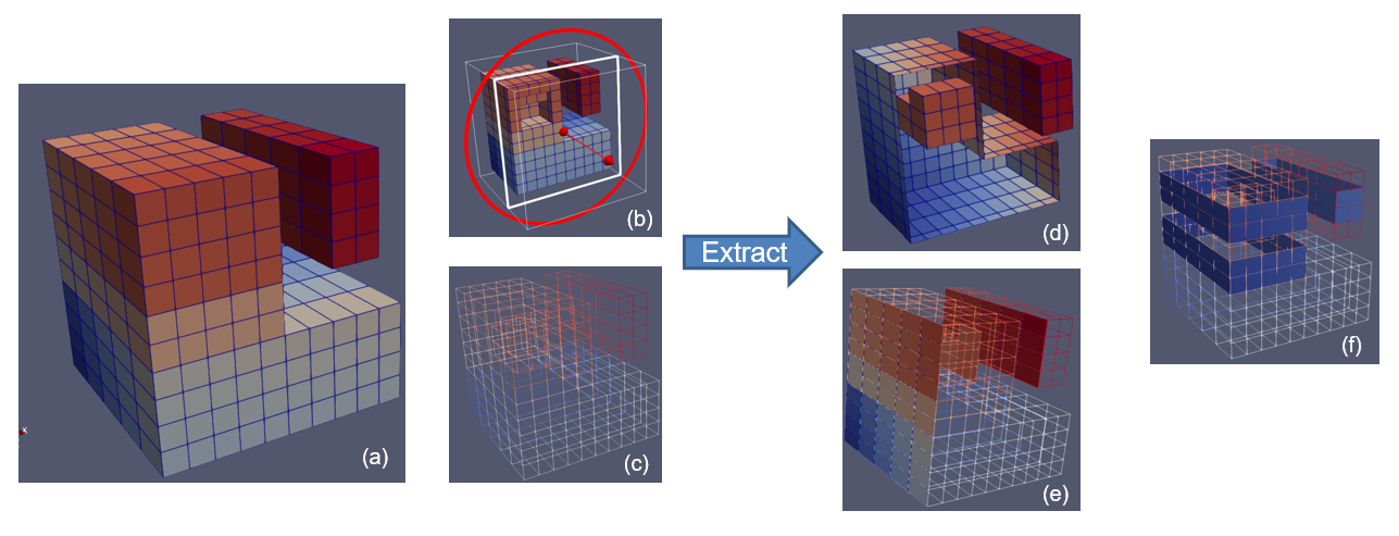
The image below exemplifies the reuslt of applying a filter function to a volumetric mesh. Image (a) shows a volumetric mesh with 3 surface borders (one hidden). Image (b) shows a transversal cut of mesh (a) showing the internal cavity. Image (c) shows the wireframe representation of the mesh. Image (d) shows a transversal cut of the extracted surfaces for a filter function that only returns true, extracting all surface faces. Image (e) shows the result of a second filter function that accepts any face whose normal vector points in the negative X direction. Image (f) shows the result of a complex filter function the uses material properties and centroid location to select several face strips.
Available d table fields are listed below. Notice that all coordinates and coordinate related calculations are done with the element's vertices only, even for quadratic elements. This is both faster and easier since it doesn't requires interpolations for interface element faces that don't have the full set of quadratic nodes. When applied over a cell side (edge or face), coordinates only include those edge / face vertices.
cellProperties table.cellAttributes table. Depending on the attribute dimension, the returned value will be either a number or a vector object.Except for very simple meshes, it is always a good idea to separate the mesh meta-data information given by the Mesh definition clause and its bulk data given by the set of node coordinates, cell geometry information, boundary data and initialization values (for both nodes and cells).
This can be done by saving that data in an auxiliary file that stores node, cell and border data into tables that are loaded by the model file through a call to the standard Lua dofile() function, much in the same way as is commonly done in the master simulation file. The only trick is to make sure that the data file returns the tables through a return clause. The example below illustrates this technique.
mySimulation_model.lua:
mySimulation_meshData.lua:
Dummy example for an heterogeneous mesh, supporting ghost nodes and using most of the above defined fields:
 1.12.0