 |
DGFemPhysics
The GeMA Discontinuous Galerkin FEM Physics Plugin
|
|
DGFemPhysics
The GeMA Discontinuous Galerkin FEM Physics Plugin
|
Discontinuous Galerkin (DG) methods can be viewed as finite element method allowing for discontinuities in the discrete trial and test spaces. From a practical viewpoint, working with discontinuities discrete spaces leads to compact discretization stencil and, at the same time, offers a substantial amount of flexibility, making the approach appealing for multi-domain and multiphysics simulations. Let a unsteady version of advection-reaction boundary condition problem, for a given finite time \(t_f>0\), consider the time evolution problem:
\begin{eqnarray*} \phi\frac{\partial c}{\partial t} + \mathbf{v}\cdot \text{grad}{(c)} + R = f & \text{in} & \Omega \times (0,t_f)\\ c = c_{\text{in}} & \text{on} & \partial \Omega_{-} \times (0,t_f)\\ c(\cdot , t = 0) = c_0 & \text{in} & \Omega \end{eqnarray*}
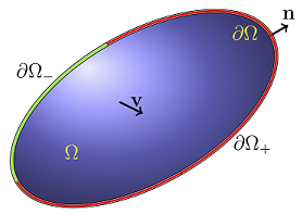
with porosity \(\phi\), advective velocity \(\mathbf{v}\), reaction term \(R\), source term \(f\), inflow value \(c_{\text{in}}\), and initial datum \(c_0\). Is it import recall that \(\partial \Omega_{-} := \left\{ x \in \partial \Omega \,|\, \mathbf{v} \cdot \mathbf{n}(x) < 0 \right\}\) where \(\partial \Omega\) represent the boundary of bound domain \(\Omega\subset \mathit{R}^{n}\) with \( n=1,2,3\). Here, the unknown function \(c:=c(x,t)\) is a scalar-valued and represents, e.g., a solute concentration.
Using the notation and concepts presented in Mathematical Aspects of Discontinuities Galerkin Methods of Daniele Di Pietro and Alexandre Ern, the discret variational form of advective-reactive problem is:
Let \(T_h\) be a regular family decomposition of \(\Omega\) into regular quadrilateral/hexahedral elements \(K\) such that \(\bigcup _{K \in T_h} K = \Omega_h \subseteq \Omega \) and given local order approximation \(p\geq 1\), find \(c_h\in C_h^p\) such that
\[ a_h(c_h,\psi) + a_\Gamma(c_h,\psi) = b_f(\psi) + b_{\text{in}}(\psi) \quad \forall \psi \in C_h^p \]
where
\[ a_h (c_h,\psi) := \sum_{K\in T_h} \int_K \left[\psi\,\phi\,\frac{\partial c}{\partial t}{-c}_h\, \mathbf v \cdot \text{grad}( \psi) + R \psi \right] dx \, , \qquad a_{\Gamma}(c_h,\psi) := \sum_{K\in T_h}\int_{\partial K} [\!| \psi |\!] \cdot \{\!|c_h \, \mathbf v|\!\}_{\text {u}} ds + \int_{\partial\Omega_+} c_h \, \mathbf v \cdot \mathbf n \, \psi ds\, , \]
\[ b_f(\psi) := \sum_{K\in T_h}\int_{K} f \, \psi \, dx \, , \qquad b_{\text{in}}(\psi) := -\int_{\partial\Omega_{-}} c_{\text{in}} \, \mathbf{v} \cdot \mathbf{n} \psi \, ds\, , \]
and
\[ C_h^p:= \left\{ c_h \in L^2(\Omega_h) \; | \; c_h\big|_K\in \mathrm{Q}_p(K) , \; \forall K \in T_h \right\} \, . \]
The above variational form is stable, but only in \(L^2(\Omega)\)-norm. The practical consequence of this can be detrimental : discontinuities in the boundary or initial datum may trigger large, non-physical oscillations in the numerical solution. In the order to design a formulation that is stable in a stronger norm, on every internal edge \(\partial K\), common to the elements \(K_1\) and \(K_2\) the upwind value of \((c\,\mathbf{v})\) is defined as:
\[ \{\!| c_h \, \mathbf v|\!\}_{\text{u}}= \left\{ \begin{array}{ccc} c_h^1 \, \mathbf{v} & \text{if} & \mathbf{v} \cdot \mathbf{n}> 0 \, , \\ c_h^2 \, \mathbf{v} & \text{if} & \mathbf{v} \cdot \mathbf{n}< 0 \, , \\ \{\!| c_h |\!\} \, \mathbf{v} & \text{if} & \mathbf{v} \cdot \mathbf{n}= 0 \, . \\ \end{array} \right. \qquad\text{(Upwind Flux)} \]
The use of a reference element, and therefore of coordinate changes, is a essential ingredient of finite element methods. Let \(\hat{K}\subset R^{n}\) and \(F\) a smooth mapping of \(R^n\) into \(R^n\), we defined \(K = F(\hat{K})\) for all \(K \in T_h\) such that for \(p\geq 1\), \( Q_p(K) := \hat{Q}_p(F^{-1}(K)) \) where
\[ \hat{Q}_p (\hat{K}):= \left\{\xi_1^i \xi_2^j\, ; \; (\xi_1,\xi_2)\in \hat{K}=[-1,1]^2\;\; \big|\;\; i,j = 0,\dots,p\right\}\quad \text{for quadrilateral elements and } \hat{Q}_p (\hat{K}):= \left\{\xi_1^i \xi_2^j\xi_3^k\, ; \; (\xi_1,\xi_2,\xi_3)\in \hat{K}=[-1,1]^3\;\; \big|\;\; i,j,k = 0,\dots,p\right\} \quad \text{ for hexahedral elements.} \]
A reference manual documenting the set of state variables and material properties expected by the plugin, along with all of its supported configuration and result options can be found here.
 1.8.15