FemProcess

Introduction

The Fem Process plugin implements both linear and non-linear solvers using the Finite Element Method. Those solvers are published as GeMA processes that can be used on the orchestration script.

Steps needed in a FEM analysis are basically the same, independently of the equations being solved. The distinction between a stress and a temperature analysis are mainly the equations that are solved to calculate local element matrices. In GeMA, the global steps of the FEM analysis are implemented by the process, while the routines used to calculate local element matrices are given by FEM physics objects.

The main entities involved in a finite element analysis are:

• The mesh defining the spatial domain;
• The set of state variables defining the degrees of freedom that will be calculated;
• The set of physics objects providing implementations for the equations to be solved;
• The numerical solver used to solve the resulting linear equation system;
• The set of boundary conditions imposed on the problem to guarantee that it has a unique solution;
• Optional contact boundary conditions for contact problems;
• The set of initial conditions for transient problems given by the actual mesh values for the referenced state variables and attributes;

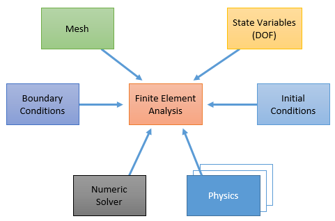
When calling a FEM process, the set of physics objects and the numerical solver are explicitly given as function parameters. The underlying mesh and boundary conditions are tied to the physics objects. State variables and initial values are tied to the mesh.

When solving single physics problems, the physics set will have a single entry. For multiphysics problems, its size depends on the strategy used by the physics plugin implementations. Hydro-Mechanical simulations, for example, are done using a single HM coupled physics while Thermo-Mechanical simulations are done by combining a mechanical physics with a thermo physics and a coupling TM physics. This behavior is specified by each physics plugin documentation.

The linear solver

The linear FEM solver is tailored for solving steady state linear FEM problems. It basically solves a \(Kx = f\) equation where the "stiffness" matrix \(K\) and the force vector \(f\) are filled by using the supplied physics objects. This solver is the basic building block for all the other solvers.

This solver can also be used for solving non-linear systems by simple fixed-point iterations. A more efficient solver based on the Newton-Raphson method is given by the non-linear solver.

The process functions exported by this solver to the orchestration environment are:

• fem.solve()
• fem.initLinearSolver()
• fem.linearStep()
• fem.linearResidual()

Their full documentation can be found here.

The transient linear solver

This solver is tailored for solving transient linear FEM problems. It basically solves a \(C\dot{x} + Kx = f\) equation where the "damping" matrix \(C\), the "stiffness" matrix \(K\) and the force vector \(f\) are filled by using the supplied physics objects. The time-domain discretization is done using an implicit schema:

\[ (C + \Delta tK)x^{n+1} = Cx^{n} + \Delta tf^{n+1} \]

Like the linear solver, this solver can also be used for solving non-linear transient systems by simple fixed-point iterations. A more efficient solver based on the Newton-Raphson method is given by the non-linear solver.

The process functions exported by this solver to the orchestration environment are:

• fem.initTransientSolver()
• fem.transientStep()
• fem.transientLinearStep()
• fem.transientLinearResidual()

Their full documentation can be found here.

The nonlinear solver

The linear FEM described above is adequate and robust, since the problems are assumed to be linear. However, many aplications in engineering problems exhibit non-linear behaviour, that must be only successfully simulated by nonlinear methods.

The process functions exported by this solver to the orchestration environment are:

• fem.run()
• fem.init()
• fem.step()
• fem.geostatic()

Their full documentation can be found here.

The nonlinear transient solver

Modeling of multiphysics problems leads in many cases to ordinary an partial differential equations which often are of nonlinear nature. Nonlinearities can be of different types, such as: geometric nonlinearity, physical nonlinearity, nonlinear boundary conditions, finite deformations, coupled problems, among others. When different fields of multiphysical interaction are coupled, for example, between solids, fluids, heat conduction in solids, etc., the formulation of complex physical problems is necessary. in all these cases the nonlinearities in each of the different field equations must be considered.

This solver is tailored for solving nonlinear transient FEM problems. It basically solves a \(C\left ( x \right )\dot{x} + K\left ( x \right )x = f\left ( x \right )\) equation where the "damping" matrix \(C\left ( x \right )\), the "stiffness" matrix \(K\left ( x \right )\) and the force vector \(f\left ( x \right )\) are filled by using the supplied physics objects. the time-domain discretization is done using the generalized \(\theta\)-method.

\[ \left ( C\left ( x \right ) + \Delta t\theta K\left ( x \right )\right ).x_{n+1} = \left ( C\left ( x \right ) - \Delta t\left ( 1 - \theta \right )K\left ( x \right )\right ).x_{n} + \Delta t\left ( \theta f_{n+1} - \left ( 1 - \theta \right )f_{n}\right ) \]

where \(\Delta t = t_{n+1} - t_{n}\) is the time step and \( \theta \) is the implicitness parameter with \(0 \leq \theta \leq 1\)

• \( \theta = 0 \) forward Euler scheme explicit
• \( \theta = 1/2 \) Crank-Nicolson scheme implicit
• \( \theta = 1 \) backward Euler scheme implicit

The default time integration considers the implicit method backward Euler scheme.

The process functions exported by this solver to the orchestration environment are:

• fem.init()
• fem.step()
• fem.geostatic()

Their full documentation can be found here.

GeMA project main page