 |
Xfem
The Xfem Plugin
|
|
Xfem
The Xfem Plugin
|
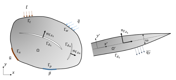
The boundary value problem considered is a two dimensional domain with a strong discontinuity, as depicted in Figure 1 (Khoei, 2015). Discontinuities are taken into account by applying the discontinuous Gauss-Green divergence theorem to the governing equations. Additionally, XFEM treats efficiently the displacement and pressure jumps caused by strong discontinuities in the model.
Integrating the product of the equilibrium and flow continuity equations, multiplied by admissible test functions over the analyzed domain, applying the discontinuous Gauss-Green divergence theorem, imposing the natural boundary conditions, and satisfying the continuity conditions on the material interface results in the weak form of the governing partial differential equations (Khoei et al, 2014). For the fractured body and the fractured domain:
\begin{eqnarray*} \int_\Omega \delta\varepsilon^T\sigma'd\Omega + \int_\Omega \delta\varepsilon^T amp d\Omega+\int_{\Gamma d}\left[\delta u \right ]^T \left(-\alpha p_Fn_{\Gamma d}\right)d\Gamma-\int_{\Gamma t}\delta u^T\bar{t}d\Gamma=0 \end{eqnarray*}
\begin{eqnarray*} \int_\Omega \nabla \delta p^Tk\nabla p d\Omega + \left ( \int_{\Gamma d} \delta p^T C p d\Gamma+\int_{\Gamma d} \delta p ^T Cp_Fd\Gamma\right )+\int_\Omega \delta p^T\alpha \nabla\dot ud\Omega+\int_{\Gamma w}\delta p^T\bar{q}d\Gamma=0 \end{eqnarray*}
\begin{eqnarray*} \int_\Omega \nabla \delta p^Tk\nabla p d\Omega + \left ( \int_{\Gamma d} \delta p^T C p d\Gamma+\int_{\Gamma d} \delta p ^T Cp_Fd\Gamma\right )+\int_\Omega \delta p_F^T\alpha \nabla\dot ud\Omega=0 \end{eqnarray*}
Where, \( \sigma' \) is the effective stress tensor; \( p \) is the average pore fluid pressure; \( m \) is the unitary components normal direction vector; \( p_F \) is the discontinuity fluid pressure; \( n_{\Gamma d} \) is the unit normal vector at the discontinuity surface; \( \bar{t} \) is the traction imposed to externanl boundary of the body; \( \bar{p} \) is the fluid flux imposed to externanl boundary of the body; \( k \) is the permeability matrix; \( C \) is the leak-off coefficient; \( k_F \) is the fracture longitudinal permeability; \( \delta \varepsilon^T , \delta u^T, \delta p^T, \delta p_F^T \) are test functions.
In addition, the integrals over the domain of the discontinuity \( \Omega' \) are performed in the local Cartesian coordinate system \( \left (x',y' \right) \) , see Fig. 1, in which the integral over the cross section of the discontinuity is evaluated by ignoring the variation of fluid pressure across the discontinuity width.
Equations are discretized in space employing the partition of unity concept via the extended finite element method, (Belytschko et al, 2009). The enriched approximations of displacement, pressures and test functions consider additional degrees of freedom \( \left( \bar{a},\bar{c} \right) \) which are multiplied by a discontinuous shape function are, (Fries & Belytschko, 2010):
\begin{eqnarray*} u\left(x,t\right)=\sum_{i\in \delta} N_{ui}^{std} \bar{u_l}\left(t\right)+\sum_{J\in\vartheta}N_{u_j}^{std}\bar{a_J}\left(t \right )H\left(x \right ) \end{eqnarray*}
\begin{eqnarray*} p\left(x,t\right)=\sum_{i\in \delta} N_{pi}^{std} \bar{p_l}\left(t\right)+\sum_{J\in\vartheta}N_{p_j}^{std}\bar{c_J}\left(t \right )H\left(x \right ) \end{eqnarray*}
Where,
\( N_{ui}^{std} \) is the standard finite element shape function;
\( \bar{u_i}, \bar{p_i} \) are the standard nodal degrees of freedom;
\(\bar{a_J},\bar{c_J} \) are the enhanced nodal degrees of freedom;
\( H(x) \) is the heaviside enrichment function;
\( \delta \) the set of all nodes in the mesh;
\( \vartheta \) is the set of nodes associated to elements completely cut by the crack.
By substituting the enriched FE approximations into the weak form equations, rearranging the integral terms, and satisfying the requirement that the weak form should hold for all kinematically admissible test functions (Mohammadnejad & Khoei, 2013), it is straightforward to obtain the discrete system of nonlinear equations:
\begin{eqnarray*}\left[K\right]\left\{ \bar{\mathbb{U}} \right\}-\left[Q\right]\left\{ \bar{\mathbb{P}} \right\}-\left[Q_{uPF}\right]\left\{ \bar{\mathbb{P_F}} \right\}=F_\mathbb{U}^{ext} \end{eqnarray*}
\begin{eqnarray*}\left[Q_T\right]\left\{\dot{ \bar{\mathbb{U}}} \right\}+\left[H+L1\right]\left\{ \bar{\mathbb{P}} \right\}+\left[S\right]\left\{\dot{\bar{\mathbb{P}}}\right\}-\left[Q_{uPF}\right]\left\{ \bar{\mathbb{P_F}} \right\}=q_\mathbb{P}^{ext} \end{eqnarray*}
\begin{eqnarray*} \left[L2^T\right]\left\{ \bar{\mathbb{P}} \right\}+\left[H_F+L3\right]\left\{ \bar{\mathbb{P_F}} \right\}+\left[Q_F\right]\left\{\dot{\bar{\mathbb{U}}}\right\}=q_{pf}^{ext}\end{eqnarray*}
The coupled equations system are solved with the implicit backward Euler scheme and the Newton-Raphson method.
The coefficient matrices in the system of discretized governing equations are defined as in Cruz (2018):
\begin{eqnarray*}K_{\beta\gamma}=\int_\Omega\left(B_u^\beta \right )^TDB_u^\gamma d\Omega \end{eqnarray*}
\begin{eqnarray*}Q_{\beta\delta}=\int_\Omega\alpha m\left(B_u^\beta \right )^TN_p^\delta d\Omega \end{eqnarray*}
\begin{eqnarray*}Q_{\beta\lambda}=\int_{\Gamma_c}\left[\left[N_u^\beta \right ] \right ]\left( \alpha n_{\Gamma_c}\right )N_{pF}^\lambda d\Gamma \end{eqnarray*}
\begin{eqnarray*}f_{\beta}^{ext}=\int_{\Gamma_c}\left(N_u^\beta \right )^T\bar t d\Gamma \end{eqnarray*}
\begin{eqnarray*}H_{\delta\xi}=\int_{\Omega}\left(B_p^\delta \right )^Tk B_p^\xi d\Gamma \end{eqnarray*}
\begin{eqnarray*}L1_{\delta\xi}=\int_{\Gamma_d}\left(N_p^\delta \right )^TcN_{p}^\xi d\Gamma \end{eqnarray*}
\begin{eqnarray*}L2_{\delta\lambda}=\int_{\Gamma_c}\left(N_p^\delta \right )^TcN_{p_F}^\lambda d\Gamma \end{eqnarray*}
\begin{eqnarray*}S_{\delta\xi}=\int_{\Omega}\left(N_p^\delta \right )^T \frac{1}{Q}N_{p}^\xi d\Gamma \end{eqnarray*}
\begin{eqnarray*}HF_{\lambda\lambda}=\int_{\Gamma_c}\left(B_{p_F}^\lambda \right )^T t_{\Gamma c}\left(2h \right )k_{Fd} \left(B_{pF}^\lambda \right ) t_{\Gamma c}^\xi d\Gamma \end{eqnarray*}
\begin{eqnarray*}L3_{\lambda\lambda}=\int_{\Gamma_c}\left(N_{p_F}^\lambda \right )^T C\left(N_{pF}^\lambda \right ) d\Gamma \end{eqnarray*}
\begin{eqnarray*}\left [ Q_F \right ]=\begin{bmatrix} E_{PFu} & E_{PFa}\\ 0 & Q_{PFu} \end{bmatrix} \end{eqnarray*}
\begin{eqnarray*}E_{\lambda\beta}=\int_{\Gamma_c}\left(N_{p_F}^\lambda \right )^T t_{\Gamma c}\left(2h \right )\alpha m \left(B_{u}^\beta \right ) t_{\Gamma c} d\Gamma \end{eqnarray*}
With \( \beta, \gamma, \delta, \xi \) being standard or enriched except for \( \lambda \) that can only be standard.
1.Belytschko, T., Gracie, R., & Ventura, G. (2009). A Review of Extended/Generalized Finite Element Methods for Material Modelling. Modell Simul Mater Sci Eng, 17(4). https://doi.org/10.1088/0965-0393/17/4/043001
2.Cruz, R. F. P. M. L. da. (2018). An XFEM element to model intersections between hydraulic and natural fractures in porous rocks. Ph.D. thesis Pontifical Catholic University of Rio de Janeiro.
3.Fries, T.-P., & Belytschko, T. (2010). The extended/generalized finite element method: An overview of the method and its applications. International Journal for Numerical Methods in Engineering, 84, 253/304. https://doi.org/10.1002/nme.2914
4.Khoei, A. R. (2015). Extended Finite Element Method: Theory and Applications. John Wiley & Sons. https://doi.org/10.1002/9781118869673
5.Khoei, A. R., Vahab, M., Haghighat, E., & Moallemi, S. (2014). A mesh-independent finite element formulation for modeling crack growth in saturated porous media based on an enriched-FEM technique. International Journal of Fracture, 188(1), 79/108. https://doi.org/10.1007/s10704-014-9948-2
6.Mohammadnejad, T., & Khoei, A. R. (2013). An extended finite element method for hydraulic fracture propagation in deformable porous media with the cohesive crack model. Finite Elements in Analysis and Design, 73, 77/95. https://doi.org/10.1016/j.finel.2013.05.005
A reference manual documenting the set of state variables and material properties expected by the plugin, along with all of its supported configuration and result options can be found here.
Several example simulations involving xfem for hydraulic fractures calculations are available at the examples directory provided with the GeMA instalation. A summary of those examples can be found here.
 1.8.15