 |
CoupledHMFemPhysics
The GeMA Coupled Hydro-Mechanical FEM Physics Plugin
|
|
CoupledHMFemPhysics
The GeMA Coupled Hydro-Mechanical FEM Physics Plugin
|
The generalized Hooke's law can be used to predict the changes in effective stresses caused in a given material by an arbitrary combination of changes in deformations \( (\Delta \varepsilon) \) as follows:
\begin{eqnarray*}\Delta \sigma' = D\Delta\varepsilon \end{eqnarray*}
where,
\( \sigma'= \begin {Bmatrix} \sigma'_{xx} & \sigma'_{yy} & \sigma'_{zz} & \tau'_{xy} & \tau'_{yz} & \tau'_{xz} \end {Bmatrix}^T \) is the tensor of effective stress;
D represents the constitutive matrix;
\( \varepsilon = \begin {Bmatrix} \varepsilon_{xx} & \varepsilon_{yy} & \varepsilon_{zz} & \gamma_{xy} & \gamma_{yz} & \gamma_{xz}\end {Bmatrix} ^T \) is the tensor of strains.
The linear isotropic elastic model is the simplest form to represent the matrix D through the consideration of only two independent elastic constants: the Bulk (K) and the shear (G) moduli of the skeleton.
\begin{eqnarray*}D=D_e=\begin {bmatrix} K+\frac{4G}{3} & K-\frac{2G}{3} & ... & 0 \\ K-\frac{2G}{3} & K+\frac{4G}{3} & ... & 0 \\ &\ddots \\0&...&G&0\\0&...&0&G \end{bmatrix} \end{eqnarray*}
Observe that this matrix can also be represented through other two elastic constants: Young's modulus (E) and Poisson's ratio ( \(\nu\)).
While elastic models are relatively simple, they cannot simulate many of the important characteristics of real rock behavior. Improvements can be made by extending these models using the theory of plasticity. Three essential ingredients are necessary to formulate an elasto-plastic constitutive model: a yield function (F), a plastic potential function (P) and hardening/softening rules. In Geomechanics, it is often convenient to work with alternative invariant quantities which are combinations of the effective stresses. A convenient choice of these invariants is to adopt the mean effective stress \((p')\), the deviatoric stress \((J)\) and Lode's angle \((\theta)\).
It is possible to establish the yield functions (F) of some constitutive models.
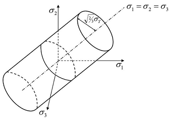
For the Von-Mises model: Figure 1.
\begin{eqnarray*}F_{VM} = J-\frac{\sigma_y}{\sqrt3} \end{eqnarray*}
Where,
\( \sigma_y \) is a material parameter representing the yield stress.
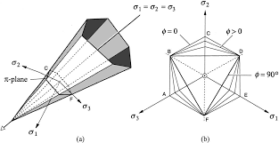
The Mohr-Coulomb model can be illustrated by the Figure 2 and equation:
\begin{eqnarray*}F_{MC} = J-\left(\frac{c'}{tan \phi'}+p'\right )\left(\frac{\sqrt3 sin\phi'}{\sqrt3 cos\theta +sin\theta sin\phi'}\right ) \end{eqnarray*}
Where,
c' is the cohesive strength;
\( \phi' \) is the friction angle.
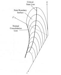
For Modified Cam-Clay model illustrated by the Figure 3 and equation: ("Working in Progress")
\begin{eqnarray*}F_{CC} = \left(\frac{J}{p'M_J}\right )^2-\left(\frac{p_0}{p'}-1 \right ) \end{eqnarray*}
Where,
\( M_J \) and \( p_0 \) are material parameters.
In most applications, those models assume that the plastic potential function is the same as the yield function (i.e. P=F). In this case, the flow rule is said to be associated. In general, the yield and plastic potential functions differ and the flow rule is said to be non-associated. The elasto-plastic constitutive matrix is given by the following equation:
\begin{eqnarray*}D=D_{ep}=D_e-\frac{D_e\left\{\frac{\partial P}{\partial \sigma}\right\} \left\{\frac{\partial F}{\partial \sigma}\right\}^TD_e}{\left\{\frac{\partial F}{\partial \sigma}\right\}^TD_e\left\{\frac{\partial P}{\partial \sigma}\right\}+A}\end{eqnarray*}
Where parameter A depends on the hardening/softening rules (e.g. perfect plasticity, strain hardening/softening plasticity or work hardening/softening plasticity).
Darcy's law relates the hydraulic flux to the hydraulic head. It postulates that the flux goes from regions of high hydraulic head to those of low hydraulic head, with a magnitude that is proportional to the hydraulic gradient, according to:
\begin{eqnarray*}v_H = -k_H\nabla H \end{eqnarray*}
where
H is the hydraulic head which is the sum of the pressure head \( (p/\gamma_f )\) and the elevation head \( z \) ;
\( k_H \) is the hydraulic conductivity of the medium;
\( v_H \) is the hydraulic flux ;
\( \nabla H \) is the gradient or vector differential operator given by:
\begin{eqnarray*}\nabla = \begin {Bmatrix} \frac{\partial}{\partial x}&\frac{\partial}{\partial y}&\frac{\partial}{\partial z}\end{Bmatrix}^T\end{eqnarray*}
The assessment of the hydraulic conductivity matrix is in general given by:
\begin{eqnarray*}k_H = k_rk_{sat} \end{eqnarray*}
Where,
\( k_r \) represents the relative permeability;
\( k_{sat} \) the matrix of saturated hydraulic conductivity of a fluid phase.
The coefficient \( k_r \) ranges between 0-1 and depends on the degree of saturation (S), which in turn is dependent on the pore fluid pressure. Those relationships are known as retention curves. Different empirical models, such as Brooks & Corey and van Genuchten models have been developed in the literature for their representation.
The relative permeability in the Brooks & Corey formulation is given by
\begin{eqnarray*}k_H = \left (\frac{S-S_r}{1-S_r}\right)^\frac{2+3\lambda}{\lambda}=\left(S^e\right)^\frac{2+3\lambda}{\lambda} \end{eqnarray*}
where,
\( S_r \) is the effective saturation;
\( S^e \) is the residual and effective saturation;
\( \lambda \) is a model parameter.
The relative permeability in the van-Genuchten formulation is given by
\begin{eqnarray*}k_r =\left(S^e\right)^\frac{1}{2} \left[1-\left(1-\left(S^e\right)^\frac{1}{m_{vg}}\right)^{m_{vg}}\right]^2\end{eqnarray*}
Where \( m_{vg} \) is a model parameter.
Under saturated conditions ( \( S^e=1 \)), the coefficient of relative permeability is equal to 1 and the saturated model is recovered.
The general form of mass balance equation for a single phase fluid flow, incorporating Darcy's law, can be expressed as follows
\begin{eqnarray*}\nabla\left(-\frac{k_H}{\gamma_f}\nabla \left(p+\gamma_{fz}\right)\right)+ \left(\frac{\alpha-\phi}{K_s}+\frac{\phi}{K_f}\right)\frac{\partial p}{\partial t} + \alpha m \frac{\partial \varepsilon}{\partial t}-\left[\left(\alpha-\phi\right)\beta_s+\phi\beta_f\right]\frac{\partial T}{\partial t}=0 \end{eqnarray*}
Where,
\( \phi \) is the porosity,
\( K_s \) is the bulk modulus of the grain solids and
\( t \) is the time.
The fluid properties are:
\( \gamma_f \) the specific weight,
\( K_f \) the bulk modulus and
\( \beta_f \) the volumetric thermal expansion coefficient.
The coefficient in the second term is often referred in the literature as Biot's modulus.
For the Coupled Hydro-Mechanics approach, based on the principle of minimum potential energy a general equilibrium equation can be written as:
\begin{eqnarray*}\delta \Delta E = \delta \Delta W- \delta \Delta L = 0 \end{eqnarray*}
Where,
\( \Delta E \) is the incremental potencial energy;
\( \Delta W \) is the incremental strain energy;
\( \Delta L \) is the incremental work done by applied loads.
Solving the terms it will give:
\begin{eqnarray*} \left [ K_G \right ]\left \{ \Delta d \right \}_{nG}+\left [ L_G\right ]\left\{\Delta p_f \right \}_{nG}=\left\{\Delta R_G \right\} \end{eqnarray*}
Where,
\begin{eqnarray*}\left [ K_G \right ]=\sum_{i=1}^{N}\left[K_E \right ]_i = \sum_{i=1}^{N} \left( \int_{Vol}\left[ B \right ] ^T\left[D'\right]\left[B \right ]dVol \right)_i \end{eqnarray*}
\begin{eqnarray*}\left [ L_G \right ]=\sum_{i=1}^{N}\left[L_E \right ]_i = \sum_{i=1}^{N} \left( \int_{Vol}\left\{m\right\}\left[B \right ] ^T\left[N_p \right ]dVol\right)_i \end{eqnarray*}
\begin{eqnarray*} \left \{ \Delta R_G \right \}=\sum_{i=1}^{N}\left \{ \Delta R_E \right \}_i = \sum_{i=1}^{N} \left[ \left( \int_{Vol}\left[N \right ] ^T\left\{\Delta F\right\}dVol\right)_i+ \left( \int_{Surf}\left[N \right ] ^T\left\{\Delta T\right\}dSurf\right)_i\right ]\end{eqnarray*}
\begin{eqnarray*} \left \{m \right\}^T=\begin {Bmatrix} 1&1&1&0&0&0 \end {Bmatrix} \end{eqnarray*}
1)Benra, F.K., Dohmen, H.J., Pei, J., Schuster, S. and Wan, B. (2011) A comparison of one-way and two-way coupling methods for numerical analysis of fluid-structure interactions. Journal of Applied Mathematics, Article ID 853560.
2)Chin, L.Y., Thomas, L.K., Sylte, J.E. and Pierson, R.G. (2002). Iterative Coupled Analysis of Geomechanics and Fluid Flow for Rock Compaction in Reservoir Simulation. Oil & Gas Science and Technology, v. 57, No. 5, 485-497.
3)Dean, R.H., Gai, x. Stone, C.M. and Minkoff, S.E. (2006) A comparison of techniques for coupling porous flow and geomechanics , Society of Petroleum Engineers Journal, 132-140.
4)Falcao, F.O.L. (2014). Hydromechanical simulation of a carbonate petroleum reservoir using pseudo-coupling. Phd. Thesis. Pontifical Catholic University of Rio de Janeiro.
5)Holman, J.P. (1989). Heat Transfer, McGraw-Hill.
6)Jaeger, J.C., Cook, N.G.W. (1979). Fundamentals of Rock Mechanics, third ed. Chapman and Hall, London.
7)Kim, J., Tchelep, H.A., Juanes, R. (2009). Stability, Accuracy and efficiency of sequential methods for coupled flow and geomechanics. Society of Petroleum Engineers, SPE 119084.
8)Kim, J., Tchelep, H.A., Juanes, R. (2011). Stability and convergence of sequential methods for coupled flow and geomechanics: fixed-stress and fixed-strain splits.
9)Kim, J., Tchelep, H.A. and Juanes, R. (2013). Rigorous coupling of geomechanics and multiphase flow with strong capillarity. Society of Petroleum Engineers, SPE 141268.
10)Mikelic, A. and Wheeler, M. (2013) Convergence of iterative coupling for coupled flow and geomechanics. Comput Geosci, v. 17, pp. 455-461.
11)Minkoff, S.E., Stone, C.M., Bryant, S. Peszinska, M. and Wheeler, M.F. (2003). Coupled fluid flow and geomechanical deformation modeling. Journal of Petroleum Science and Engineering, v. 38, pp. 37-56.
12)Manoharam, N. and Dasgupta, S. P. (1995) Consolidation analysis of elasto-plastic soil Computers & Structures. v. 54, pp 1005-1021.
13)Murad, M.A., Borges, M., Obregon, J.A. and Correa, M. (2012). A new locally conservative numerical method for two-phase flow in heterogeneous poroelastic media. Computers and Geotechnics, v. 48, pp. 192-207.
14)Potts, D.M. and Zdravkovic, L. (1999). Finite element analysis in geotechnical engineering – Theory. Thomas Telford Publishing, London.
15)Quispe, R.J.Q. (2012). Three-dimensional analysis of hydromechanical problems in partially saturated soils. Phd. Thesis. Pontifical Catholic University of Rio de Janeiro.
16)Scrimieri, D., Afazov, S., Becker, A., Ratchev, S. (2014). Fast mapping of finite element field variables between meshes with different densities and element types - Adv Eng Softw, v. 67, pp. 90–98.
17)Settari, A. and Mourits, F.M. (1998). A coupled reservoir and geomechanical simulation system. Society of Petroleum Engineers, SPE 50939.
18)Settari, A. and Walters, D.A. (1999) Advances in coupled geomechanical and reservoir modeling with applications to reservoir compaction. Society of Petroleum Engineers, SPE 74142.
19)Udai, B.R. Prasetyo, H., Tang, H.K. and Cua, C.L. (2014) On the use of a full-field geomechanical model to influence and optimize field development decisions: case study from an HPHT field in south China Sea. Society of Petroleum Engineers, SPE 170614-MS.
20)Zienkiewicz, O.C. Paul, D.K., and Chan, A.H.C. (1988). Unconditionally stable staggered solution procedure for soil-pore fluid interaction problems. Int J. Numer Methods Eng, v. 26(5), pp. 1039-1055.
A reference manual documenting the set of state variables and material properties expected by the plugin, along with all of its supported configuration and result options can be found here.
Several example simulations involving Coupled Hydro-Mechanics for calculations are available at the examples directory provided with the GeMA installation. A summary of those examples can be found here.
A reference manual documenting the set of state variables and material properties expected by the plugin, along with all of its supported configuration and result options can be found here.
 1.8.15