 |
CoupledHMFemPhysics
The GeMA Coupled Hydro-Mechanical FEM Physics Plugin
|
|
CoupledHMFemPhysics
The GeMA Coupled Hydro-Mechanical FEM Physics Plugin
|
The Dual Porosity Dual Permeability (DPDP) Coupled Hydraulic Mechanics Finite Element physics plugin is responsable for providing implementation for model to simulate fluid flow in naturally fractured reservoirs that can be used with the Fem process to solve coupled transient mechanic hydraulic problems, both in 2D and 3D. The DPDP models were extended to deformable fractured media to study possible impacts of geomechanical parameters on flow inside the fracture, porosity and permeability (Wilson & Aifantis, 1982; and Elsworth & Bai, 1992, Bagheri and Settari, 2008; Lemonnier, 2010; Bertrand et al, 2017; Rueda et al, 2019). Considering a negative compression, the relationship between total stress and effective stresses in dual porosity media can be defined as:
\begin{eqnarray*}\sigma_m = \sigma'_m -\alpha_mp_m\end{eqnarray*}
\begin{eqnarray*} \sigma_f=\sigma'_{fr}-\alpha_{fr} p_{fr}\end{eqnarray*}
Where the subscripts \( m \) and \( fr \) refer to matrix and fracture respectively; \( p_m \) and \( p_{fr} \) are the fluid pressures in the matrix and in the fractures, respectively, and \(\alpha_m\) and \(\alpha_f\) are the Biot coefficients. It is important to keep the equilibrium of the stress at local level \(\sigma = \sigma_m = sigma_f\)
The total strain is the sum
\begin{eqnarray*}\varepsilon_{m fr} = \varepsilon_m + \varepsilon_{fr} \end{eqnarray*}
where \( \varepsilon_m \) and \( \varepsilon_{fr}\) are matrix and fracture strains, respectively. The constitutive relationships between strain and effective stress are:
\begin{eqnarray*}\varepsilon_m = C_m:\sigma'_m \end{eqnarray*}
\begin{eqnarray*}\varepsilon_{fr} = C_{fr}:\sigma'_{fr} \end{eqnarray*}
where \(C_m \) and \( C_{fr}\) are the compliance tensor of the matrix and fracture (Bai, 1999). The equations that govern the deformation of solids and the phase of the fluid in dual porosity of a pore-mechanical problem can be expressed as:
\begin{eqnarray*}\nabla (D_{m fr}:\varepsilon_m-D_{m fr}:C_m:\alpha_mp_m-D_{mfr}:C_{fr}:\alpha_{fr}p_{fr})+f=0 \end{eqnarray*}
\begin{eqnarray*}\frac{k_m}{\mu}\nabla^2p_m +D_{mfr}:C_m:\alpha_m:\frac{\partial}{\partial t}\varepsilon+\beta_m \frac{\partial p_m}{\partial t}+\omega (p_m-p_{fr}+q_m=0 \end{eqnarray*}
\begin{eqnarray*}\frac{k_{fr}}{\mu}\nabla^2p_{fr} +D_{mfr}:C_{fr}:\alpha_{fr}:\frac{\partial \varepsilon}{\partial t}+\beta_{fr} \frac{\partial p_{fr}}{\partial t}-\omega (p_m-p_{fr}+q_{fr}=0 \end{eqnarray*}
In these expressions \( D_{mfr}\) is the equivalent elasticity tensor of the matrix/fracture system; \( f \) represents the external force vector; \( k_m\) and \( k_{fr}\) stand for the permeability of the rock matrix and fracture system; \( \mu \) is the dynamic viscosity of the fluid; \( t\) is the time; \( \beta_m \) and \( \beta_{fr}\) are the relative compressibility representing deformability of the fluid and solid; and \( q_m\) and \( q_{fr}\) are the fluid flow in the matrix and in the fracture system, respectively. \( \omega \) is the shape transfer factor which controls the fluid transfer between matrix blocks and fracture system. Warren and Root (1960) defined the shape transfer factor as
\begin{eqnarray*}\omega=\frac{k_m}{\mu} \frac {4a(a+2)}{s^2} \end{eqnarray*}
where \(a\) = 1,2,3 are the normal sets of fractures. For three orthogonal fractures } \( a\) = 3, the spacing \(s\) can be defined as:
\begin{eqnarray*}s =\frac{3s_x s_y s_z}{s_x s_y+s_y s_z+s_x s_z} \end{eqnarray*}
Kasemi et al (1976) present a shape transfer factor based on Warren and Root (1960) as follow:
\begin{eqnarray*}\omega=\frac{4}{\mu}\left [ \frac{1}{s_x^2}+\frac{1}{s_y^2}+\frac{1}{s_z^2} \right ] \end{eqnarray*}
Subsequently, this shape transfer factor is generalized for anisotropic models as:
\begin{eqnarray*}\omega=\frac{4}{\mu}\left [ \frac{k_{mx}}{s_x^2}+\frac{k_{my}}{s_y^2}+\frac{k_{mz}}{s_z^2} \right ] \end{eqnarray*}
Recently, Rueda et al (2020) devolped an enhanced shape factor to multi-block domains formed by different fracture sets with arbitrary orientations. Therefore, the shape factor \( \omega \) for a rock block domain Figure 1, assuming a pseudo (quasi) steady-state condition, can be expressed as:
\begin{eqnarray*}\omega=\frac{1}{V} \sum_{i=1}^{nfaces}\left[\frac{A}{d_c}k_{mn} \right ]_i \end{eqnarray*}
where \( V \) is the volume of the matrix block; \( A \) is the area of the open fracture surface; \( d_c \) is the distance from the centroid of the block matrix to fracture surface \( i \); \( k_{mn} \) is the rock permeability normal to the open fracture plane, and \( nfaces \) is the number of block faces in contact with open fractures.

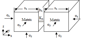
Fluid flow in a single fracture may be described by plate analogy, where a fracture is idealized as a constant planar aperture. As Figure 2 shows, the permeability through a set of parallel fractures with spacing \( s\) and aperture \(b\) is given by:
\begin{eqnarray*}k_{fr0}=\frac{b^3}{12s} \end{eqnarray*}
where \(k_{fr0}\) is the initial permeability of the fracture set. Various models define strain and permeability relations in fractured media (Elsworth, 1989; Bai et al, 1997; Zhang et al, 2006).
The example work adopts a strain and permeability relation based on a relative displacement theory of interface elements (Rueda, 2013). From Eq. (15), the variable permeability in -i direction due to aperture changes in -i direction for a single set of fractures can be defined as follows
\begin{eqnarray*}k_{fr-k}=\frac{(b_{0i}+\Delta b_i)^3}{12s_i} \end{eqnarray*}
where \( \Delta b_i \) is the relative displacement variation of the fractures in -i direction calculated in terms of the total strain as:
\begin{eqnarray*}\Delta b_i=\left [\frac{E}{E+s_ik_n} \right ] \varepsilon_{mfr} \end{eqnarray*}
\( E \) is the elasticity rock module, \( k_n \) is normal stiffness, and \( s \) is the spacing between fractures.
For generalized cases, the permeability tensor of the fracture system in a global coordinate \( (x, y, z) \) is defined as:
\begin{eqnarray*}k_{fr}=\sum_{i=1}^{nfaces}\left[R^T k_{fr}^{l} R \right ]_i \end{eqnarray*}
where \( k_{fr}^{l} \) is the permeability tensor of a fracture set in a local system, which is dependent on its aperture \( b \) and spacing \( s \) as follows:
\begin{eqnarray*}k_{fr}^{l}=\begin {bmatrix} \frac{(b_{0}+\Delta b)^3}{12s} & 0 & 0 \\ 0 & \frac{(b_{0}+\Delta b)^3}{12s} & 0 \\ 0& 0 & \frac{(b_{0}+\Delta b)^3}{12s} \end{bmatrix} \end{eqnarray*}
and \( R \) is the rotation matrix defined as:
\begin{eqnarray*}R =\begin {bmatrix} sin(\theta) & cos(\theta) & 0 \\ cos(\phi) cos(\theta) & -cos(\phi) sin(\theta) & -sin(\phi) \\ -sin(\phi) cos(\theta) & sin(\phi) sin(\theta) & -cos(\phi) \end{bmatrix} \end{eqnarray*}
where \( \theta \) is the strike angle, and \( \phi \) is the dip angle.
A reference manual documenting the set of state variables and material properties expected by the plugin, along with all of its supported configuration and result options can be found here.
 1.8.15