 |
GeMA
The GeMA main application
|
|
GeMA
The GeMA main application
|
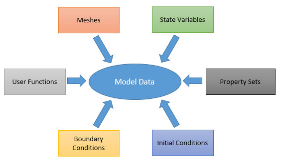
As seen on section I - Basic GeMA concepts, the model data describes what will be simulated. In our example problem, it should describe the discretized plate, along with its material properties and boundary conditions. For a GeMA simulation, the model data is composed of five types of objects (Figure 6): state variables, property sets, user functions, meshes and boundary conditions. It can also specify initial values, needed for transient problems.
State variables represent model degrees of freedom, corresponding to values that are calculated by the simulation. They are global entities that can be associated with several meshes. When a state variable is associated with a mesh, space is reserved for storing a value for that state variable, per mesh node.
In our example, the problem needs a scalar state variable to represent the temperature. It can be declared as
where the id is the name that will be used to reference this state variable throughout the model, description is a meta-data field that describes its meaning and format defines the numeric format that will be used when printing or saving temperature values to text format files.
The unit attribute specifies that the data associated with state variable T will be stored in degrees Celsius and that will be the default unit for printing and saving temperature values. If the physics that will process the temperature calculation needs values in another unit (Kelvin, for example) the data will be converted automatically. Whenever a state variable is used by a physics, it will check if its unit is compatible with the expected unit, so if you declare that your temperature state variable is measured in meters, the thermo physics will not accept that variable. An empty unit is always compatible with any other unit.
The set of available units is extensive and can be configured as described in Working with units. Most common units are accepted, including common unit multipliers and any combination of known units. When defining a unit, the following points, among others, should be observed:
There are other field options that can be added to a StateVar definition and they will be explored further on while treating node and cell attributes, but two of them are worth mentioning in the state variable context: dim and defVal. The first defines the state variable dimension for the creation of vector-valued variables. The second gives the initial value for the variable if not initialized in another way (if not given, that default initialization value will be equal to 0.0). As an example, the definition below defines a vector valued state variable with 3 dimensions and initialized with a value of 0.5 mm in x and y.
When creating a FEM simulation, the set of needed state variables, their default names and their dimensions are generally driven by the set of used physics objects (this information can be found in each physics plugin documentation), and that brings up a question of why do we need to declare the used state variables, instead of inferring them by the set of used physics. There are several reasons for that. The first is that this inference can be difficult in a scenario with multiple meshes, multiple physics and the relationship between them defined dynamically during the orchestration. Second, that this inference might not be possible with generic physics objects that can apply their calculations to different kinds of physical concepts. One such physics could be an implementation of the advection-conduction equation, which can be applied, for example, over temperatures or concentrations. The third and last reason is that some of the state variable important attributes, such as its initial value and unit, are not tied to the physics and would need a place to be defined anyway.
Property sets are data tables used mainly to store physical material properties. Each line represents a material and each column one physical property of that material. If a mesh is associated with a property set, each mesh cell will store one property table line index.
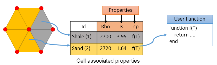
Figure 7 shows a mesh with 6 triangle cells and a property set table, storing properties for two rock types: shale and sand. Orange cells are "sand" cells, and so they store index material '2', while gray cells ar "shale" cells. All orange cells share the same set of rock properties.
Naturally, property sets can be used to store any kind of cell-associated data, and not only material properties. Fabrication parameters, such as the cross-section area for a truss element, are one such example. Since the cross section of a truss is independent of its physical properties, and a model can have several trusses made of the same material, but with different cross sections, a mesh can be associated with several property sets, one for its physical properties and another for its fabrication parameters in this example. If that was not the case, there would need to be several lines in the property set table with the same physical properties, each for one cross section value.
When a mesh is tied to several property sets, each mesh cell will store a line index per property set. Similarly to state variables, property sets are global simulation objects that can be associated with several meshes.
For the tutorial example problem, the temperature calculation requires the knowledge about the plate's conductivity for the steady state analysis and also its density and specific heat capacity for the transient analysis. Since this is a 2D problem, the plate's width should also be provided. To illustrate the possibility of working with several property sets, we will construct our model with one thermal properties table and another with fabrication properties. They can be declared by the following code:
Like state variables and any other GeMA object declaration, a PropertySet has a description and an id that will be used to reference this object in the model. Since property sets are implemented by plugins, its declaration should explicitly name the plugin that will be used to interpret this property set. This is done by the typeName field, which will appear in every plugin based declaration. In this example, the standard property set plugin, GemaPropertySet, will be used.
The material properties set has three columns for storing the plate's conductivity, density, and specific heat capacity declared inside the properties field. The syntax (and the semantic) used for defining those columns in lines 7, 8 and 9 is exactly the same as the one used before by state variables, and also the same that will be used by attribute definitions (the full set of options will be presented shortly while detailing attributes).
Property values are given inside the values field, which is a Lua table with one subtable for each line in the property set. Inside that subtable, values are tied to their columns by name. If a column does not have an explicit value, it will assume the default value for that column. Since our example model has just one material, the values table has just one entry (line 12). If it had more materials, line 12 would have its structure duplicated for each material as seen in the next example.
Later, when relating each cell to its material, the line index in the values subtable can be used to identify each one, remembering that in Lua table indexing starts at 1 (in C++, indices start at 0 and the GeMA framework follows each language convention). Alternatively, material lines can be given an identifier that will be later used to tie a cell to a material. This can be done as in the example below, where the names MatA, MatB and MatC were given to a set of three materials.
Figure 7 shows property values for the heat capacity tied to a user function. Details about functions will be given shortly. In our heat conduction problem, they could be used to specify, for example, a non-linear property where the conductivity or the heat capacity are functions of the temperature. Another usage example would be to specify a plate width varying with mesh position.
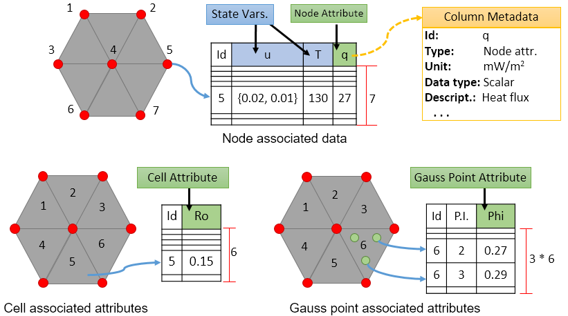
Attributes are data sets that can be used to store derived results calculated by the simulation, such as the heat flux in a temperature simulation or stresses in a mechanical simulation. They can also be used to store any kind of input or calculated user data, being associated with mesh nodes, mesh cells or even with element integration (Gauss) points (Figure 8).
Since our proposed heat conduction simulation can have its results compared to an analytical solution, we are going to add an attribute for calculating the observed error in each mesh node. Instead of adding a single attribute that calculates the error, for illustration purposes we are going to add two attributes to the mesh. The first will calculate the expected temperature in each node and will have its value filled while mesh nodes are initialized. The second one will be a user function that calculates the absolute difference between the analytical and the FEM calculated temperatures.
Attributes are not real objects that can be declared as state variables or property sets. Instead, they are part of the mesh definition as will be seen on section V - Model data 2. Nevertheless, to better organize our simulation model, their declarations will be grouped in an auxiliary table that will later be referenced by the mesh. As already said, their syntax is equal to the one seen before for state variables and properties.
The above code declares two attributes: Tana and Err. Notice that the Err definition includes two additional fields: functions and defVal. The first tells GeMA that Err values can be user declared functions. The second tells that, in the absence of an explicit initialization, the attribute should be filled with a reference to the user function called errf.
Possible fields that can be added to an attribute, state variable or property definition are:
"lxc" where l is the number of lines and c the number of columns in the matrix;functions, allocMode and/or allocStrategy. If that is the case, values will be stored as doubles, the default if this option is missing. Accepted values are "double", "float", "int32", "int16", "byte", "uint32", "uint16" and "ubyte";defVal = {0.0, 1.0, 0.0} will initialize it with a normalized vector pointing in the y direction. If a scalar value is given, it will be used to fill all of the vector dimensions. For matrices, the initial value can be either given by a table of tables or linearized by column major format (the same used in the FORTRAN language), so, for a 2x2 matrix, both defVal = {11, 21, 12, 22} and defVal = { {11, 12}, {21, 22} } statements correspond to the matrix \(\begin{pmatrix} 11 & 12 \\ 21 & 22 \end{pmatrix}\). If the attribute allows function values, the default value can be a string with the function name. If this field is not filled, the default value will be equal to zero (or a vector/matrix filled with zeros in all its dimensions);"sparse" for telling GeMA that most data values will be equal to the default value, "full" for telling that most of the data is different from the default or "auto" for telling that the data is "full", but space should be allocated only after the first write to the data set of a value different from the default. This is the default behaviour (except for state variables that only accept "full" values) and can produce great memory economy when attributes are created and not used or for attributes whose sole value is its default, a common pattern when working with user functions;allocMode is equal to "sparse". Currently unimplemented. Accepted values are: "auto";printf() syntax, allowing the user to specify the field width, precision and format type. A ‘format = '8.2f’‘ statement means that the formatted value will have at least 8 characters and 2 decimal values. Allowed format specifiers are 'f’ (for decimal floating point format), 'e' (for scientific notation format) and 'g' (corresponding to 'f' or 'e', whichever is shortest);"geometry" means that this attribute has values for geometry nodes only. A value of "ghost" means that this attribute has values for ghost nodes only and a value of "both"means that it stores values for all node types. When absent, a geometry storage is used;true, an unlimited number os past values will be enabled. A positive number greater than 1 defines the exact number of saved states that will be used in a rolling history pattern. A value of 2, for example, means that the current value and the last one are saved. When a new value is calculated, the current one becomes the last one and the last one is discarded (see Figure 9).constMap = {A = 1, B = 2, C = 3} statement means that if the string "A" is used to initialize a value, it will be translated into the value 1. Those statements are valid for scalar attributes only. If an attribute allows both constant maps and function definitions, the translation process takes precedence over function name recognition. Constants defined in a constMap can be used in a defVal statement.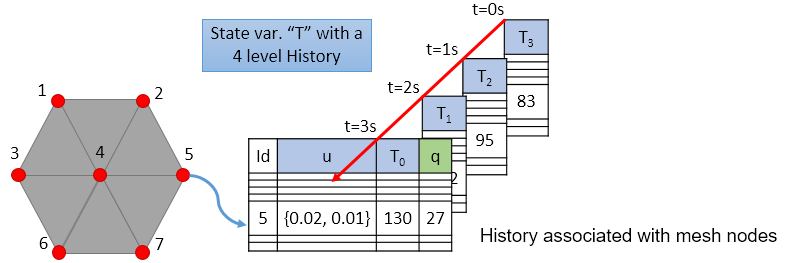
User functions are functions that can be used to enhance attributes, properties and boundary condition values with a dynamic behavior. They can be implemented either in Lua or in C++. In this tutorial, only the former will be treated.
There are two kinds of user functions: node functions and cell functions. As their names imply, node functions can be used to provide values for node attributes and cell functions for cell properties, cell attributes, and Gauss attributes. The code below shows the declaration of the errf node function, responsible for calculating values for the Err attribute, defined earlier. A cell function follows a similar syntax, being named CellFunction instead of NodeFunction.
On the above code, the parameters field is used to define the set of parameters that will be provided to the user function. For the example problem, the error evaluation function expects to receive the value of the Tana node attribute (the expected analytical temperature), and the value of the T state variable (the calculated temperature), as given by the parameters src fields.
The method field contains the Lua function that will be called whenever the attribute's value is requested for a specific mesh node. As specified by the parameters field, when called, this function will receive the values of the Tana attribute and the T state variable, both evaluated on the mesh node. Function parameters must follow the same order in which they appear on the parameters table (their names, on the other hand, can be different from the source names - only the position counts). On this example, the function only needs to calculate the absolute difference between the values, using for that the standard Lua function math.abs().
On our example, both function parameters are scalar values, but vector and matrix parameters are also accepted. They are received by the method function as Lua tables and can be indexed as such. Matrices are linearized into a table following a column major format, as seen before while the defVal field was presented. It is expected that the function result should be consistent with the dimension of the attribute that the function is tied to. Like received parameters, vector and matrix results should be returned as a Lua table.
When declaring a function parameter, the following fields are accepted:
"coordinate": The parameter will receive a table with node coordinates;"time": The parameter will receive the current simulation time;"dt": The parameter will receive the elapsed time between the current time and the last simulation iteration;"nodeid": The parameter will receive the node id;"meshid": The parameter will receive the mesh name;{src = "coordinate", dim = 2} the resulting value passed to the function will be a scalar value with the y node coordinate, instead of a vector;Cell functions support almost the same set of fields, the main difference being the available options for the src field:
"time": The parameter will receive the current simulation time;"dt": The parameter will receive the elapsed time between the current time and the last simulation iteration;"cellid": The parameter will receive the cell id;"meshid": The parameter will receive the mesh name;"ipoint": The parameter will receive a table with the current integration point Cartesian coordinates;"nipoint": The parameter will receive a table with the current integration point natural coordinates;When a cell function requests a node attribute or a state variable as a function parameter, the cell function evaluation will generally occur on an integration point, and the GeMA framework interpolates the node values on that point, passing this interpolated value as the parameter. On Figure 7, the heat capacity property (cp) is defined as a function of the node temperature. When the analysis process queries the cp value over an element integration point, the value of the state variable T is interpolated based on element nodal values and the resulting temperature passed as the parameter to f(T). All this process is done automatically by the framework in a transparent way. Notice that this process can be recursive since function parameters can be user functions themselves.
The interpolation method can be controlled by the interpType field and its default behavior is to do a shape function interpolation for element based meshes and an inverse distance squared interpolation for cell meshes (see V - Model data 2 for a distinction between cell and element mesh types). See the User functions documentation for additional details.
One important additional point to keep in mind is that user functions are evaluated only when the attribute associated with this function has its value queried. In our tutorial example, that means that if the value of the Err attribute is never queried, the errf function will never be executed. That query can occur explicitly on the orchestration script, by the user asking for the value of the Err attribute for a mesh node, or implicitly if the attribute is included in a call to a process that prints or saves data to a file.
Go to the next section, previous section or return to the index.
 1.8.15