 |
GeMA
The GeMA main application
|
|
GeMA
The GeMA main application
|
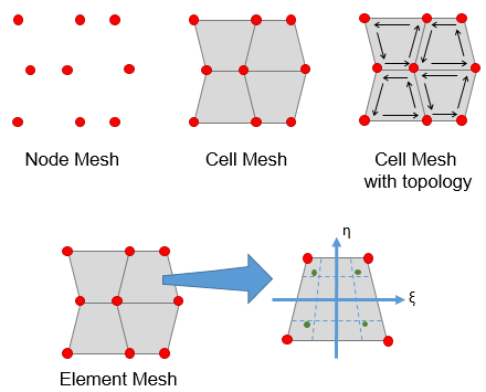
The GeMA framework is not committed to any particular discretization method. Since different methods require different types of domain discretization, the framework applies a hierarchical approach in order to be flexible and try to support several of those methods. In GeMA, domain discretizations are loosely called "meshes", even if the discretization consists of a simple point cloud, as in "mesh free" methods.
For the framework, a mesh is composed by a set of nodes, each tied to its spatial position and, possibly associated with a dataset. This is a very open definition that does not imply any kind of topology.
Inheriting from a mesh, the frameworks second support level is a cell mesh. A cell defines a partition of the global spatial domain and is represented in 1D by a segment, in 2D by an area and in 3D by a volume. In general, those cells are disjoint and their union represents the whole spatial domain. Each cell is formed by an ordered set of nodes that collectively define its border geometry. The schema defining how many nodes exist in a cell and their organization defines the cell type.
The third level in GeMA's mesh hierarchy is the element mesh, supporting the finite element method. It extends the cell concept by associating each cell to an interpolation function (shape function) and to a set of integration points. Figure 10 illustrates these concepts, that can be further extended to support other needs.
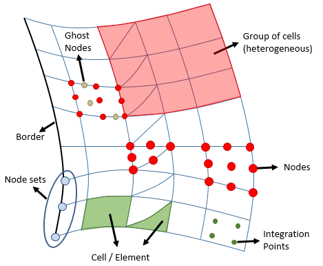
A GeMA simulation can contain multiple meshes, and those meshes can store heterogeneous cell types. Figure 11 shows an example of a heterogeneous mesh and its related entities. They are:
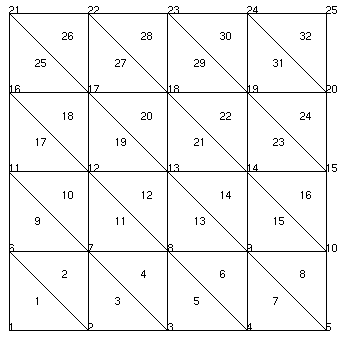
To solve our proposed heat conductivity problem, the plate will be discretized into a structured mesh composed by triangle elements. Our first mesh will be composed of 25 nodes and 32 triangles as shown in Figure 12. The Lua code to create this simple mesh is shown below.
Looking at the mesh typeName field, we can see that it is implemented by the standard mesh plugin, identified by its name "GemaMesh". The ".elem" part of the typeName field is used to tell the mesh plugin that the desired mesh is an element mesh. Other options are ".nodes" for node only meshes and "cell" for cell meshes.
The coordinateDim and coordinateUnit fields are used to inform the mesh that this is a 2D mesh and that node Cartesian coordinates are expressed in centimeters. The stateVars field ties this mesh to the previously declared temperature state variable. If the simulation involved more variables, they would be listed inside this subtable.
Node attributes and material properties are tied to the mesh by the nodeAttributes and cellProperties fields. The latter references the names of both property sets defined previously. Remember that a simulation can have several meshes, so each one could be tied to different state variables, property sets, and node attributes, making this fields necessary. If our simulation needed cell attributes or Gauss attributes, their definitions would be given in the cellAttributes and gaussAttributes fields.
The 'real' mesh definition is given by fields nodeData and cellData. The first is responsible for providing the list of mesh node coordinates while the second is responsible for defining element geometry. Node data is given by the MeshNodeCoordinates Lua table and its syntax is straightforward: each table entry contains a subtable with node coordinates.
The MeshElements Lua table is used to provide cell geometry and also to bind mesh elements to their respective materials. Since our problem mesh is homogeneous, and all cells share the same material, this table has only one entry, a subtable that basically informs that our mesh is composed by linear triangle elements (cellType = "tri3"), that the list with element geometry is given by the MeshTriList table and that all cells are tied to the first entry in the MatProp and FabProp property sets. The auxiliary MeshTriList table gives the set of nodes used to form each mesh triangle. Nodes are organized in a CCW fashion as required by GeMA tri3 elements.
If the mesh had heterogeneous elements or if we desired to create named element groups, the MeshElements table would have more entries, as shown in the example below, consisting of three sets of elements. The first is a set of triangles, the second a set of quadrilateral elements named "quads", and the third a second set of triangles. If two table lines use the same group name, both element sets will be merged into the same named element group.
Notice that in the above example no material properties were tied to the cell groups. In fact, the material definitions seen previouslly on the tutorial problem mesh declaration, are really default values that are used only if a material is not associated directly with a mesh element during its geometry definition. That can be done by following the node set in the element definition with a material declaration, as in the example below where the first shown triangle is tied to the named "shale" material and to the third fabrication property, while the second triangle will be tied to the default fabrication property defined in the MeshElements table.
The last important point in our mesh declaration is the definition of mesh borders. Those are needed for boundary conditions later on and are given by the boundaryEdgeData field that references the MeshBorders Lua table. If this was a 3D problem, boundary faces would have been defined by the boundaryFaceData field. The MeshBorders table follows a now familiar syntax, with one sub-table for each named border. In those subtables, the id field gives the border name while the cellList field provides a list with (cell number, border number) pairs. As an example, the first MeshBorders subtable specifies that the top border is composed by the second edge of cells 26, 28, 30 and 32, as can easily be seen in Figure 12. Please remember that edge numbering follows the order in which the cell nodes were defined. For a linear triangle, the second edge is the edge between the second and third given nodes. See the Element types documentation for a reference.
The standard mesh plugin accepts several other field options that were not covered in the previous example. Their meaning and some usage examples can be found on the standard mesh plugin reference documentation.
Unless explicitly given, attributes and state variables are initialized with their default value, as given by the defVal field in their respective declarations, or with 0.0 in the absence of that field.
In our heat conduction simulation, we must properly initialize the Tana attribute with the analytically calculated temperature for each node (Err doesn't need special initialization since all nodes will reference the same user function given by defVal).
This initialization can be done in the same table used to define node coordinates by following them with initial values for node attributes and state variables, in that order (and in their respective declaration orders). It is not necessary to provide initialization values for all attributes and state variables, but if you want to give an initial value to the second attribute and not to the first, the former must be replaced by a nil value. Vector and matrix values are represented by subtables with the initial values for each dimension. Functions are represented by a string with the function name. Strings can also be used if the initialized value has a constMap used for translating strings into values. The same technique can be used to initialize cell attributes: just add the initial values after the geometry node list.
To add initial values for Tana, we begin by creating a Lua function that calculates the analytical temperature solution at a given coordinate following the equation defined in section II - Example problem, then we add a call to that function in each of the node coordinate table entries, as seen below.
An easier alternative, that uses the fact that the simulation model is really a Lua script, can be seen in the code below that uses a loop to add values to the original node coordinates table MeshNodeCoordinates. The Lua construct "for i=1, #MeshNodeCoordinates do" is a loop that runs from i = 1 to the number of entries in the MeshNodeCoordinates table, increasing i by one at each step.
Since our example problem is laid over a regular domain and our desired simulation mesh is a structured mesh, instead of manually creating our node and cell lists, as we have done earlier in a boring and error prone way, we can create Lua functions capable of building the contents of the MeshNodeCoordinates, MeshTriList and MeshBorders tables. As an additional bonus, since those functions can be made to receive as parameters the desired number of mesh nodes in each direction, we end up being able to easily parameterize the size of the mesh used to solve the problem. The mesh creation functions are given below.
In fact, since creating regular meshes is so common, the Mesh Lib set of auxilliary functions provides an out of the box alternative for the above code (see the heat conduction example for further explanations and a working code):
When running the GeMA application, it is possible for the user to send parameters to the simulation (see section VII - Running your simulation). Those parameters are accessed in the simulation file by using the global variable userParams. By using this variable, instead of a constant value, the mesh size can be chosen by the user when running the simulation. For that, we just need to replace the first two lines of the previous script with:
Finally, the last missing part in our model data are the boundary conditions. For the GeMA framework, a boundary condition object stores a set of boundary conditions, all sharing the same type and mesh. It also stores a set of properties with values for each single condition. Those properties are described in the same way as any attribute and their values can also be user functions, allowing for an easy way to represent boundary conditions that change over time.
The meaning of each of those properties is collectively identified by the object type field, which is interpreted by the physics object that will ultimately make use of this boundary condition. When creating a model, the physics plugin is the authority that defines which are the available boundary condition types and their required properties. The plugin options documentation can be found here.
A condition also stores where it should be applied. All conditions in the object are tied to the same kind of application point. Available options are nodes, cells, cell edges or cell faces. When applying a boundary condition to nodes, edges or faces, border names declared inside the mesh definition can be used as the application point.
Our heat conduction problem requires a Dirichlet boundary condition that prescribes fixed temperature values over the plate border nodes. For that, the thermo physics plugin recognizes the "node temperature" boundary condition type, which has a single property "T" storing the prescribed node temperature. The thermo physics also supports other boundary conditions types, as can be seen in its documentation.
The code above shows the needed boundary condition object to complete our simulation model data. The mesh field ties this boundary condition to the problem mesh (remember that a generic GeMA simulation can have several meshes). The properties field defines the set of properties used by the boundary condition using the now familiar syntax used on attribute definitions.
The nodeValues field is used to tie property values to mesh nodes. Each of its entries is a subtable that begins with a node number or a border name, followed by values for the declared properties. When the node is given by a border name, the value set is applied to all nodes in that border.
For boundary conditions tied to cells, the cellValues field should be used. For this kind of condition, the application point, given as the first value in each table line, should be a cell number. For edges and faces, the edgeValues and faceValues fields should be used. For them, the application point must be a border name.
Go to the next section, previous section or return to the index.
 1.8.15