Conceptually, our example simulation problem, described by the model data created on previous sections, can be solved by several different numerical methods. As seen on section I - Basic GeMA concepts, the solution method describes how the problem should be solved. In our heat conduction example, its role will be to guide the GeMA framework into solving the heat equation by the finite element method.

Figure 13: Solution method

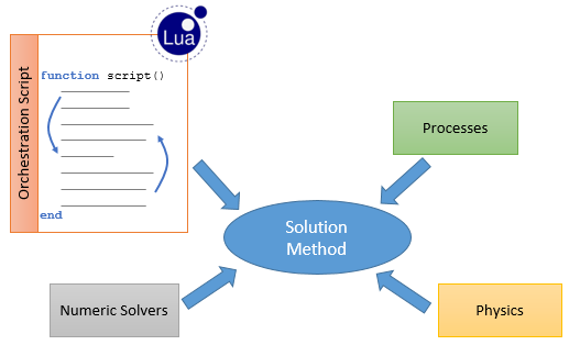
For a GeMA simulation, the solution method is composed of four main entities (Figure 13):

Orchestration script: The orchestration script is the heart and soul of the solution method and one of the main reasons for the GeMA flexibility. Written in the Lua language, it defines, through series of function calls and language constructions (loops, conditions, etc), the order in which processes will be executed during the simulations, thus providing its main loop. Given Lua's expressiveness, the orchestrator can execute operations as complex as needed.
Processes: Processes are the basic unit used for describing the solution. They can be written in C++ or in Lua through user defined functions. Generally, they are high-level primitives that describe a complete action, such as the execution of a step in a finite element analysis, the transfer of data from one mesh to another, saving a dataset, etc. When a process is executed by the orchestrator, it can receive several other model entities as parameters. In particular, analysis processes usually make use of physics and numerical solvers.
Physics: Physics objects are responsible for helping analysis processes build the equation system that will be solved. In general, the process is responsible for the core of the analysis algorithm, while the physics implements aspects that are particular to a specific equation. In a FEM analysis, for example, physics cooperate to produce element local matrices that will be merged into the global matrix by the FEM process.
Numeric solvers: Numeric solvers are the objects responsible for solving the equation systems that often arise from the analysis algorithms. Different solvers can use different methods to solve those equations.

Processes

In a broad way, the execution of a simulation can be seen as being composed by the execution of a series of processes that exchange data between them, cooperating to achieve the desired final result. Among others, the GeMA framework includes processes for:

Executing finite element method (FEM) simulations;
Transferring data between different meshes;
Reading and writing mesh files with their associated data;
Writing information to log files;
Integration with external programs (through Lua processes).

The FEM process implements the analysis method required for the solution of our example problem. The main entities involved in a finite element analysis are given in Figure 14. They are:

Figure 14: Fem process

The mesh defining the spatial domain;
The set of state variables defining the degrees of freedom that will be calculated;
The set of physics objects providing implementations for the equations to be solved (see below);
The numerical solver used to solve the resulting linear equation system;
The set of boundary conditions imposed on the problem to guarantee that it has a unique solution;
The set of initial conditions for transient problems;

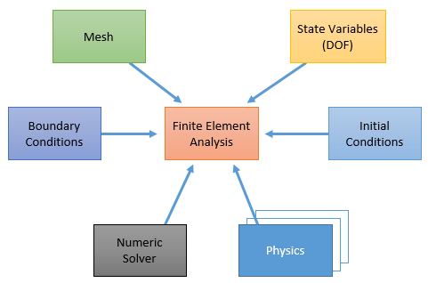
Steps needed in a FEM analysis are basically the same, independently of the equations being solved. The distinction between a stress and a temperature analysis are basically the equations that are solved to calculate local element matrices. In GeMA, the global steps of a FEM analysis are the process, while the routines used to calculate local element matrices are the physics.

Numeric solvers

Numeric solvers are implemented in GeMA by plugins. The standard numeric solver uses the Armadillo linear algebra package, that in turn uses the SuperLU library to solve symmetric or unsymmetric sparse linear systems of equations through a direct LU decomposition method.

NumericalSolver {
  id          = 'solver',
  typeName    = 'ArmadilloSolver',
  description = 'Direct matrix solver',
}

The code above declares the numerical solver that will be used in our example problem. It simply selects the Armadillo solver plugin (typeName = "ArmadilloSolver"), which doesn't needs any further configuration options.

Physics

Physics are also implemented in GeMA by plugins. The code below declares the thermo physics object required by the FEM process to solve the heat equation. It selects the standard thermo plugin (typeName = "ThermoFemPhysics") and fills some required fields for FEM processes.

PhysicalMethod {
  id       = 'HeatPhysics',
  typeName = 'ThermoFemPhysics',
  type     = 'fem',
  mesh = 'mesh',
  boundaryConditions = {'Border temperature'},
}

The type field tells GeMA that this is indeed a physics suitable for use with the FEM process. The mesh field binds it to the mesh over which the fem process will be executed. If several physics are needed, all of them must reference the same mesh. Finally, the boundaryConditions field binds the physics to the set of boundary conditions applied to the problem solution. This field is a table and can list more than one condition.

These fields are common to every FEM physics. On our example problem, no other specific options are needed. Available options can be found on the thermo plugin documentation and include, for example, options to enable heat flux recovery or internal heat generation.

Orchestration script

The orchestration script is always given by the ProcessScript() function. Running a GeMA simulation is equivalent to executing this Lua function inside the framework environment. Inside the orchestration script, processes are executed by calling them as Lua functions, independently if they were defined in C++ by a plugin or by a user given Lua function. The orchestration script for the steady state simulation is pretty simple and given below.

function ProcessScript()
  -- Solve the simulation using the FEM process
  fem.solve({'HeatPhysics'}, 'solver')
  -- Print results
  print('Calculated results:')
  io.printMeshNodeData('mesh', {'coordinate', 'T', 'Tana', 'Err'}, 
                       {header_title=true, eval_functions=true})
  
  -- Save results to a Neutral file
  io.saveMeshFile('mesh', './steadyStateCond', 'nf', {'T', 'Tana', 'Err'})
  -- Save results in Vtk format
  dofile('$SCRIPTS/vtklib.lua')
  vtkLib.saveMeshFile('mesh', {'T', 'Tana', 'Err'}, nil, './steadyStateCond')
end

The first process call, fem.solve(), executes a linear FEM analysis as a single step. It receives as parameters the set of physics objects used in the simulation, identified by their names, and the numeric solver used to solve the resulting linear equation system. This function can optionally receive other tables with additional process options, as can be seen in the linear fem process documentation.

The call to the io.printMeshNodeData() process simply prints data associated to mesh nodes. The first parameter consists of the mesh name, followed by a table that includes the set of node attributes and state variables that should be printed. The special name coordinate asks that an additional column with node coordinates should also be printed. The last parameter is a table with printing options. The eval_functions option is needed to tell the process that the functions tied to the Err attribute should be evaluated and the resulting value printed. Without this flag, the function name would be printed instead. More options can be found on the io process documentation.

Finally, the call to the io.saveMeshFile() is responsible for saving data to a file. It receives as its first parameter the mesh name, followed by the file name, its type ("nf" means that a neutral file will be created) and by a table with the set of node attributes and state variables to be saved, much as the one passed to the print process.

The VtkLib set of auxiliary functions can be used to write results in the Vtk file format, for post-processing with the Paraview application. The library is loaded with the use of the dofile() function and the file saved by the call to vtkLib.saveMeshFile().

For the transient case, another script is needed. For greater flexibility, the outer time loop is given by the orchestration and the FEM process is called once for each time step. Its code is given below.

function ProcessScript()
  -- Init the FEM solver for a transient simulation
  local solver = fem.initTransientSolver({'HeatPhysics'}, 'solver')
  local dt   = 0.001 -- Time step
  local endt = 0.2   -- End simulation time
  local nsteps = endt / dt
  -- Initialize the neutral file that will receive simulation results
  local file = io.prepareMeshFile('mesh', './transientCond', 'nf', {'T'})
  -- Load VtkLib to enable saving results in the Vtk format
  dofile('$SCRIPTS/vtkLib.lua')
 
  for i=1, nsteps do
    print(string.format('Beggining iteration %d - t = %.3f s', i, i*dt))
    setCurrentTime(i*dt)
    -- Run a simulation step
    fem.transientStep(solver, dt)
    -- Save timestep results
    io.addResultToMeshFile(file, i*dt) 
    vtkLib.saveMeshFile('mesh', {'T'}, nil, './transientCond', {state = i, stateTime = i * dt}) 
  end
  io.closeMeshFile(file)
end

At line 4, the fem analysis solver is initialized by a call to the fem.initTransientSolver() process. Its parameters are the same as the ones passed to fem.solve(), but instead of processing the simulation, this call now tells the FEM process that a transient simulation will begin and that further calls to run simulation steps will be made. The process returns a handle that stores the iterative simulation context and that should be passed as a parameter in further calls to the FEM process. This handle is stored on the solver local variable.

On lines 6 through 8, the script defines the used time step (1ms) and the simulation duration (0.2s) and calculates the number of needed time steps nsteps. In line 11, the io.prepareMeshFile() call initializes the file that will receive simulation results at each time step. Its parameters are the same as the ones passed to io.saveMeshFile() in the previous script. It also returns a handle to be passed while adding results to the file. The VtkLib is also loaded.

Line 16 is the main simulation loop, iterated nsteps times. It repeatedly executes a simulation step by calling fem.transientStep(), passing as parameters the handle obtained at line 4 and the elapsed simulation time between this call and the previous one. The loop is completed by saving the current results to file by calling io.addResultToMeshFile(), and by saving a new Vtk file for this time step (in Vtk, each step must be saved to a different file with a numeric suffix added automatically by vtkLib.saveMeshFile()). Finally, after the simulation ended, the neutral file result file is closed by a call to io.closeMeshFile().

The call to setCurrentTime() at line 19 is not a process call, but an internal GeMA function used to tell the framework about the current time. This function is not really needed in this simulation since no user functions depend on time parameters. It is included here as a good practice.

Go to the next section, previous section or return to the index.