 |
GeMA
The GeMA main application
|
|
GeMA
The GeMA main application
|
The first set of examples form a basic tutorial on how to build GeMA simulation models, illustrating both basic and some advanced techniques that can be applied on several other modelling scenarios. Those examples where created to complement the explanation given on the basic GeMA tutorial and should be followed on the same order as presented here.
Other sections on this page presents several examples illustrating some of the GeMA capabilities with both syntetic and real test cases conducted by the Geomechanics group at the Tecgraf Institute.
All the simulation models and the accompanying presentations are available on the "examples" folder installed together with the GeMA applilcation.
The last section on this page links to a set of slides and examples presented during the GeMA-ERAS training meeting for Shell collaborators on september, 24th, 2020.
| Steady state heat conduction on a square plate | |
|---|---|
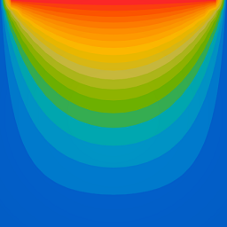
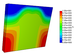
| This tutorial example presents a steady state analysis of heat conduction on a square plate subjected to Dirichlet boundary conditions. Its main objectives are to show how to strucuture a GeMA model, how to create a simple mesh, setup material values, setup a prescribed temperature boundary condition, create user functions to validate analytical and numerical results and create a simple orchestration procedure to execute a FEM analysis. Main file: Temperature\SteadyStateHeatConduction.lua |
| Transient heat conduction on a square plate | |
|---|---|
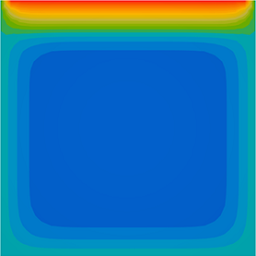
| This tutorial example presents a transient analysis of heat conduction on a square plate subjected to Dirichlet boundary conditions. Its main objective is to show how to transform the steady state analysis of the previous example into a transient analysis. Main file: Temperature\TransientHeatConduction.lua |
| Transient conduction on a heated rod | |
|---|---|
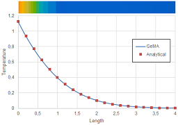
| This tutorial example simulates the heat conduction on an insulated rod with a heat influx on one of its tips, comparing the numerical results to an analytical solution. Its main objective is to further illustrate new boundary condition types by applying a Neumann boundary condition. It also shows how to create time-dependent user functions. Main file: Temperature\HeatedRod.lua |
| Temperature profile for a set of sedimentary layers | |
|---|---|
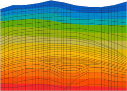
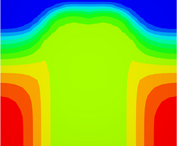
| This tutorial analyzes the temperature profile for a set of sedimentary layers subjected to a heat flux at their base and a prescribed surface temperature. It is composed by four examples with increasing functionalities. The first one does a simple steady state analysis. The second introduces porosity dependencies and non-linearities to the model materials. The third presents a transient simulation for a surface temperature boundary condition that changes with time and the fourth changes the implementation of the porosity initialization from serial to a parallel one. The main objective of this four examples is to show how some complex models can be created by combining user provided functions with advanced orchestration techniques . Main files: Temperature\BasinLayers1.lua, BasinLayers2.lua, BasinLayers3.lua and BasinLayers4.lua |
| Phase change by the effective heat capacity method | |
|---|---|
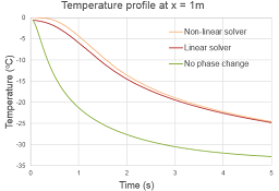
| This tutorial example presents a phase change analysis for a solidification problem, solved by using the effective heat capacity method and the non-linear FEM solver. The main objectives of this example are to give an introduction on how to use the non-linear FEM solver and to show how to track results at a given node during the simulation. Main file: Temperature\Solidification.lua |
| MeshLib tutorial | |
|---|---|
| This tutorial presents several examples of meshes that can be build by the MeshLib set of Lua scripts. Its main objective is to exemplify how to create 2D and 3D "grid like" meshes, as well as how to add interface elements to any 2D mesh and how to save meshes to a model file. Main file: MeshLib\meshLibExample.lua |
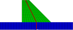
| Coupled Thermo-Mechanical analysis for a heated bar | |
|---|---|
| This examples analyses the heat conduction on a bi-material bar, subjected to heating on a small part of its bottom, coupled with thermal stress calculation. Main file: CoupledTM\BendingBar.lua |
| Modelling reservoir production | |
|---|---|
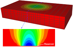
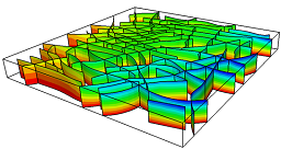
| This example illustrates the fluid flow and geomechanical behavior of a soft reservoir within a stiff region after 12-years of production. Main file: Subsidence\3D\coupledHMRes3.lua |
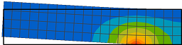
| 2D Uncoupled subsidence analysis and reservoir compaction | |
|---|---|
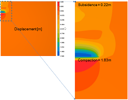
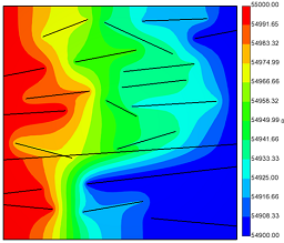
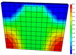
| This example illustrates an uncoupled analysis of surface subsidence and compaction of an oil reservoir located at the North Sea basin. Main file: Subsidence\2D\Subsidence_UC.lua |
| 2D Fully coupled subsidence analysis and reservoir compaction | |
|---|---|
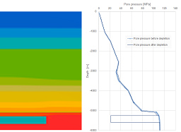
| This example illustrates a fully coupled analysis of surface subsidence and compaction of an oil reservoir located at the North Sea basin. Main file: Subsidence\2D\Subsidence_FC.lua |
| Multispecies reactive transport example | |
|---|---|
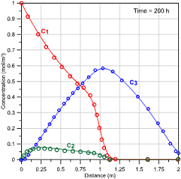
| This example presents a reactive transport analysis on a rectangular plate subjected to Dirichlet (prescribed concentration) boundary conditions and multiple species with linear reaction rates. Main file: ReactiveTransport\multispeciesReactiveTransport.lua |
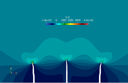
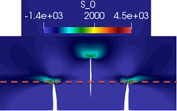
| 2D Fault reactivation | |
|---|---|
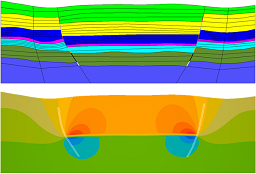
| This example presents a fault reactivation analysis of a a multi layer porous media with two main natural fractures, submitted to an hydraulic injection at the reservoir. Main file: FaultReactivation\2D\faultReactivation.lua |
| 2D Consolidation for fractured porous media | |
|---|---|

| This example presents a 2D coupled hydro-mechancal simulation for the consolidation of a naturally fractured reservoir using interface elements to represent the fractures. Main file: DiscreteFracture\2D\DFMkvar.lua |
| 2D Fluid flow in fractured porous media | |
|---|---|
| This example presents a rectangular porous media under in-situ conditions, subjected to a pore pressure gradient in the x direction. Main file: DiscreteFracture\2D\naturalFractures2D.lua |
| 3D Consolidation for fractured porous media | |
|---|---|
| This example presents a 3D coupled hydro-mechancal simulation for the consolidation of a naturally fractured reservoir using interface elements to represent the fractures. Main file: DiscreteFracture\3D\DFM3Dkvar.lua |
| 3D Fluid flow in fractured porous media | |
|---|---|
| This example presents a block of fratured porous media under in-situ conditions, subjected to a pore pressure gradient in the x direction. Main file: DiscreteFracture\3D\naturalFractures3D.lua |
| 2D Double porosity, double permeability on a fractured reservoir | |
|---|---|
| This example presents a coupled hydro-mechanical simulation of a naturally fractured reservoir using the dual porosity, dual permeability model. Main file: DualPorosityDualPermeability\2D\DPP-kvar.lua |
| 3D Double porosity, double permeability on a fractured reservoir | |
|---|---|
| This example presents a 3D coupled hydro-mechanical simulation of a naturally fractured media using the dual porosity, dual permeability model. Main file: DualPorosityDualPermeability\3D\DPDP-PTop.lua |
| 3D Dam seepage | |
|---|---|
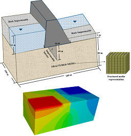
| This example presents a dam seepage problem, modeled as a 3D coupled hydro-mechanical simulation with natural fractures represented using the dual porosity, dual permeability model. Main file: DualPorosityDualPermeability\3D\DAM-DPP-DFN.lua |
| Hydraulic fracture propagation in permeable porous media using the KGD model | |
|---|---|
| This example presents a coupled Hydro-Mechanical analysis of the propagation of a fracture on an initially pressurized borehole using the KGD model. Main file: InterfaceHydraulicFracturing\hydDrivenKGD.lua |
| KGD analytical model in K-vertex propagation regime | |
|---|---|

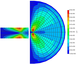
| This example presents a transient XFEM analysis of a single hydraulic fracture on a square plate, with results compared to the KGD analytical solution. Main file: XFEMHydraulicFracturing\KGD.lua |
| Single hydraulic fracture entering another layer with symmetric / asymmetric stress contrast | |
|---|---|
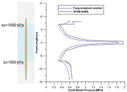
| This set of examples presents a transient XFEM analysis of a single hydraulic fracture entering another layer with symmetric and asymmetric stress contrast, with results respectively compared to Simonson and Fung analytical solutions. Main files: XFEMHydraulicFracturing\Simonson.lua and Fung.lua |
| Three simultaneous / sequential hydraulic fractures with a homogeneous stress state in a single layer | |
|---|---|
| This set of examples presents a transient XFEM analysis of three simultaneous and sequential hydraulic fractures, with an homogeneous stress state and fracture spacings of 7 and 20m. Main files: XFEMHydraulicFracturing\SimHF7.lua, SimHF20.lua, SeqHF7.lua and SeqHF20.lua |
| Three simultaneous hydraulic fractures entering another layer with symmetric stress contrast | |
|---|---|
| This set of examples presents a transient XFEM analysis of three simultaneous hydraulic fractures entering another layer with symmetric stress contrast and varying fracture spacings of 7 and 20 m. Main files: XFEMHydraulicFracturing\SimHF7SC.lua and SimHF20SC.lua |
| 1D Dissolution of a simple fracture using interface elements | |
|---|---|
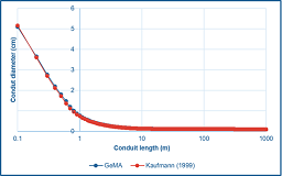
| This example presents the early evolution of a karst aquifer, modelled as a conduit. Its main objective is to show how to create a multiphysics simulation where one of the physics is implemented wholly in Lua and integrated with another GeMA physics through the global simulation loop. Main files: RockDissolution\simpleKarstEvolution.lua |
| 2D Evolution of a karst aquifer | |
|---|---|
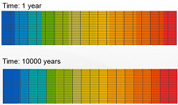
| This example presents the early evolution of a vertical karst aquifer due to the dissolution process along fractures represented by interface elements. Its main objective is to show how to create a multiphysics simulation where one of the physics is implemented wholly in Lua and integrated with another GeMA physics through the global simulation loop. Main files: RockDissolution\conceptualKarst2D.lua |
| 2D one-way HM coupling with upscaling and using an external simulator | |
|---|---|
| This example presents a one-way HM coupling simulation in 2D involving an upscaling process and the use of an external simulator. Its main objective is to show how to interface with external simulators and how to orchestrate an upscaling process. Main files: CoupledHMExternalSimulator\CoupledHMExternalSimulator.lua |
This set of examples where used during the GeMA-ERAS training meeting for Shell collaborators on september, 24th, 2020.
 1.8.15