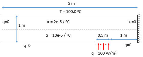
To complete our tutorial, this section presents a simple multiphysics problem coupling temperature and stress/deformation calculations. The simulated scenario is given in Figure 17, where a bar is fixed on its right side and left free to move in the other directions. The top border is kept at a constant temperature of 100.0 degrees Celsius while the other borders are isolated, with the exception of a small segment at the bottom border that is heating the bar with a heat flux of 100W/m2. The bottom half of the bar has a thermal expansion factor alpha five times bigger than the top half, forcing the bar to bend up while heated at the bottom.

Figure 17: Coupled Temperature-stress problem

Since by now the reader should already be able to understand a GeMA model, only parts of it are presented here with comments only on relevant constructions. In particular, the mesh generation is not included. It uses the Mesh Lib functions to create a regular grid mesh, assigning different materials to the top and bottom halfs of the grid. The complete code for the simulation can be downloaded at the following link:

Coupled temperature-stress: Zip file containing the three Lua files for the coupled Thermo-Mechanical simulation.

Model Data

Since our simulation now includes also deformation analysis, the set of state variables includes deformations on the x and y directions through a vector state variable, as well as the temperature.

StateVar{id = 'T', description = 'Temperature', unit = 'K', format='8.5f'}

StateVar{id = 'u', description = 'Displacements', dim = 2, unit = 'm', format='8.4f'}

The stress physics calculates the stress tensor components sxx, syy and sxy both at the nodes and at Gauss points. Since on this problem we desire to present stress results in terms of principal stresses, their values can be calculated by user functions provided by the Stress Functions Lib.

dofile('$SCRIPTS/stressFunctionsLib.lua')
-- Declares user node functions for calculating principal stresses using the stress functions lib
stressFunctionsLib.useNodeFunction('sigma1n')
stressFunctionsLib.useNodeFunction('sigma2n')
-- Declares user cell functions for calculating principal stresses on Gauss points using the stress functions lib
stressFunctionsLib.useCellFunction('sigma1')
stressFunctionsLib.useCellFunction('sigma2')

To enable deformation calculations, the property set now includes the materials elasticity modulus and Poisson ratio. The thermal expansion factor is also given. Notice that now the value set contains two rows, one for the top part of the bar and another for the bottom one.

PropertySet
{
  id          = 'MatProp',
  typeName    = 'GemaPropertySet',
  description = 'Material parameters',
  properties  = {
    {id = 'k',     description = 'Conductivity',      unit = 'W/(m.K)'},
    {id = 't',     description = 'Element thickness', unit = 'm'},
    {id = 'E',     description = 'Elasticity modulus'},
    {id = 'nu',    description = 'Poisson ratio'},
    {id = 'alpha', description = 'Thermal expansion factor',  unit = '1/K', format = '.6f'},
  },
  values = {
    {id = 'normal', k = 1.0, t = 0.01, E = 1e6, nu = 0.3, alpha = 2e-5},
    {id = 'high',   k = 1.0, t = 0.01, E = 1e6, nu = 0.3, alpha = 10e-5},
  }
}

This simulation requires three different boundary conditions. The first one, Tbc1, applies a fixed temperature condition to the top of the bar. The second one, Tbc2, applies a fixed heat flux condition to heat a bar segment on its bottom. Notice that the prescribed heat flux value is negative since heat is entering the cells. Finally, the third boundary condition, ubc, is used to prescribe a zero node displacement for nodes at the bar's right border.

BoundaryCondition {
  id   = 'Tbc1',
  type = 'node temperature',
  mesh = 'mesh',
  properties  = {
    {id = 'T',  description = 'External temperature applied on the node', unit = 'K'},
  },
  nodeValues = {
    {'topBorder', 100},
  }
}
BoundaryCondition {
  id   = 'Tbc2',
  type = 'surface flux',
  mesh = 'mesh',
  properties  = {
    {id = 'q',  description = 'Heat flow', unit = 'W/m2'},
  },
  edgeValues = {
    {'bottomHeatedBorder', -100},  -- Negative since heat is entering the element
  }
}
BoundaryCondition {
  id   = 'ubc',
  type = 'node displacements',
  mesh = 'mesh',
  properties  = {
    {id = 'ux',  description = 'Fixed node displacement in the X direction', defVal = -9999},
    {id = 'uy',  description = 'Fixed node displacement in the Y direction', defVal = -9999},
  },
  nodeValues = {
    -- border,        ux,  uy
    {'rightBorder',   0.0, 0.0},  -- Nodes fixed in x and in y
  }
}

Solution method

This multiphysics simulation requires a set of three physics for temperature calculation, deformation calculation and for the coupling of both of them. Some points worthy of notice are:

The temperature physics now includes two boundary conditions;
The mechanical physics and the coupling physics both include a suffix ".xxx" after the plugin name. This suffix informs the plugin of the kind of analysis that will be done, much like the ".elem" suffix informed the mesh plugin about the desired mesh type;
The mechanical physics includes a name translation field called properties. This is needed since this physics expects the element width to be a property named w and our model names it as t, the name expected by the temperature physics;
The stressMode option tells the physics that stresses should be recovered at both nodes and Gauss points;
The reference temperature for the material is given by the referenceT field.

-- Physics for temperature calculation
PhysicalMethod {
  id       = 'HeatPhysics',
  typeName = 'ThermoFemPhysics',
  type     = 'fem',
  mesh = 'mesh',
  boundaryConditions = {'Tbc1', 'Tbc2'},
}
-- Physics for displacement and stress calculation
PhysicalMethod {
  id       = 'StressPhysics',
  typeName = 'MechanicalFemPhysics.PlaneStress',
  type     = 'fem',
  mesh = 'mesh',
  boundaryConditions = {'ubc'},
  properties = {h = 't'},  -- Stress phisics expects width to be called 'h'
  stressMode = 'both',
}
-- Coupling physics
PhysicalMethod {
  id       = 'TempStressPhysics',
  typeName = 'CoupledTMFemPhysics.PlaneStress',
  type     = 'fem',
  mesh = 'mesh',
  properties = {h = 't'}, 
  referenceT = 100,        -- Reference temperature for the material
  stressMode = 'both',
}

The orchestration script is very similar to the one used in our previous heat conduction example. Notice that now the first parameter to fem.solve() includes the set of three physics defined above.

When calling the io.printMeshNodeData() process, notice that it includes node stresses (S) calculated by the mechanical physics and that this attribute was not included in the mesh definition (see the simulation files). When recovering stresses, the mechanical physics will add this attribute to the mesh automatically if it was not defined by the user. In a similar way, the io.printMeshGaussData() process is used to print information recovered on Gauss points.

Finally, the io.saveMeshFile() process now receives a second table with the set of Gauss attributes to be saved and a third with specific options for the neutral file format, enabling the inclusion of a deformation section in the file.

function ProcessScript()
  -- Solve the problem using the FEM method with a temperature physics, a stress physics 
  -- and a coupling physics
  fem.solve({'HeatPhysics', 'StressPhysics', 'TempStressPhysics'}, 'solver')
  print('')
  print('Calculated results:')
  -- Print calculated node data
  io.printMeshNodeData('mesh', {'T', 'u', 'S', 's1', 's2'}, 
                       {header_title = true, eval_functions = true})
  -- Print calculated Gauss data                        
  io.printMeshGaussData('mesh', {'S', 's1', 's2'}, 
                        {header_title = true, eval_functions = true})
  -- Save data to a Neutral file
  io.saveMeshFile('mesh', './tempStress', 'nf', {'u', 'T', 'S', 's1', 's2'}, 
                  {'S', 's1', 's2'}, {saveDisplacements=true})
  -- Save results in Vtk format
  dofile('$SCRIPTS/vtklib.lua')
  vtkLib.saveMeshFile('mesh', {'u', 'T', 'S', 's1', 's2'}, nil, './tempStress')
end

Results

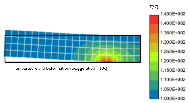
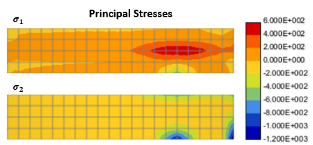
Running the simulation will produce a neutral file that can be opened in the Pos3D software. Figure 18 shows the bar deformation together with the resulting temperature distribution. Figure 19 shows the resulting principal stresses.

Figure 18: Temperature and deformation results

Figure 19: Principal stresses results

Go to the next section, previous section or return to the index.